Machine Learning is nothing but creating the machines or software which can take its own decisions on the basis of previous data collected. Technically speaking, machine learning involves ‘explicit’ programming rather than an ‘implicit’ one:
Machine learning is divided into three categories viz.
- Supervised Learning
- Unsupervised Learning
- Reinforcement Learning.
When you have an immense amount of data and you do not know what it contains, then the best approaches are to apply the algorithms of unsupervised learning like PCA (Principal Component Analysis), tSNE, SVMs.
The data visualization of such huge data can lead you to make important decisions when you have a clear picture of the data in front of you. The more complex the data, more are the dimensions.
Dimensions can be defined as a single entity among the data. Example in the debris of data of images, numbers, alphabets, clothes, shoes, beverages every single entity is accountable for a single dimension among all the dimensions. Like in this instance only we have a total of six dimensions. Here’s how:-

So in total sums to six dimensions.
Now, suppose one person hands over to you a truck of all the above data in a bag, how will you know which entity is which one! This is not where the story ends, all the IT firms now have data in a drastic amount that even they can’t pick or classify the data.
The data comprises of structured data, unstructured data, semi-structured data and what not.
So now here, the businesses hire people who have expertise in Mathematics, Machine Learning who know the puzzles of Linear algebra, Calculus, Probability, Statistics, etc. to understand and recognize the patterns in data.
If we consider the above example I would apply t-SNE (t-Distributed Stochastic Neighbour Embedding) model or algorithm to visualize or classify the data. The only reason I’m preferring t-SNE on top of PCA is that the PCA’s approach is confined to linear projection rather than the tSNE which can even capture the non-linear dependencies in the data.
Moreover, PCA is applied to preserve the overall variance of the dataset. The global covariance matrix is practiced to study the data in PCA, otherwise, there is no other option to reduce such a high dimensional data at least in the PCA model.
Constraints that binds LLE or Kernel PCA or Isomap
One way is to opt for the local structure. Actually, this one puts efforts to map the high dimensions onto low dimensional space. The low dimensional space is for 2D or 3D. This is the gap between the data points.
The above holds the definition of tSNE, then what are LLE or Kernel PCA or Isomap. Well, these are the algorithms meant for nonlinear dimensionality reduction and manifold learning.
Locally Linear Embedding acronymed as LLE goes far to the density modeling approaches unlike PCA. LLE provides the consistent set of global coordinates over the entire manifold. Apart from looking for an embedding LLE maintains the distances from every point or node to the most closer neighbor.
Similarly, ISOMAP is also one of the manifolds and dimensionality reduction algorithm. The only drawback of this is that it is way too slow. Diffusion maps are created at a turtle rate plus the maps can not untangle the Swiss Roll for a single value of a Sigma function.
That is why tSNE is more preferred as it tackles all the above problems easily.
Here’s the code to help you with. I’m writing in jupyter notebook but you can choose whatever IDE you prefer. Here’s the git link.
import numpy as np
import seaborn as sns
import matplotlib
import pandas as pd   # data processing, CSV file I/O (e.g. pd.read_csv)
from sklearn.decomposition import PCA
from sklearn.manifold import TSNE

sns.set_style("darkgrid", {"axes.facecolor": ".95"})

data = pd.read_csv('wine.csv')
data.head(5)
data.head(0)

Or to see only the first row that has all the features:
data = pd.read_csv('wine.csv')
data.head(0)
Alcohol Malic_Acid Ash Ash_Alcanity Magnesium Total_Phenols Flayanoids Nonflavanoid_Phenols Proanthocyanins Color_Intensity Hue OD280
X = data.loc[:, "Total_Phenols":"Customer_Segment"]

y = data.Ash
data.shape
(178,14)
pca = PCA(0.95)
X_pca = pca.fit_transform(data)

pca.components_.shape
pca.explained_variance_ratio_

array([0.99808763])
tsne = TSNE()
X_tsne = tsne.fit_transform(X_pca[:17])
matplotlib.rcParams['figure.figsize'] = (10.0, 10.0)
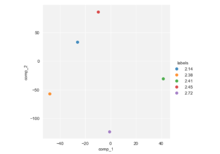
proj = pd.DataFrame(X_tsne)
proj.columns = ["comp_1", "comp_2"]
proj["labels"] = y
sns.lmplot("comp_1", "comp_2", hue="labels", data=proj.sample(5), fit_reg=False)
So, all this wraps up and leaves us with one decision that machine learning does have its some charm that overwhelms the data scientists.
If someone needs more clearance or need to know the technicalities of Machine Learning, then Stanford Machine Learning course quenches this thirst. Plus, the course also clarifies the mathematical concepts which later nourishes the decision power of an individual to decide which model is best suited for what type of data.