Ten months after part 1 of spatial regression in R (oh my gosh where did these months go?), here is a (hopefully long-awaited) second part this time using INLA, a package that is handy in many situations.
What this will be about
There are many different types of spatial data, and all come with specific models. Here we will focus on so-called geostatistical or point-reference models. Basically, you collected some informations in different locations and want to account for the fact that locations closer together are more likely to show similar values than locations further appart.
In part 1, we saw how to fit spatial regression of the following form:
yi∼N(μi,σ)
where i index the different lines in your dataset, y is the response variable, μ is a vector of expected values and σ is the residual standard deviation.
μi=Xi∗β+u(si)
the expected values depend on some covariates that are in the design matrix X, these get multiplied by some coefficient to estimate (the β's) plus a spatial random effect u that depend on location si of the data point.
The crucial part in these models is in estimating the spatial random effect, most of the time it is modelled as a multivariate normal distribution:
u(si)∼MVN(0,Σ)
and the variance-covariance matrix (Σ) is populated using the Matern correlation function:
cov(i,j)=δ∗Matern(dij,κ)
the covariance between any two locations in the dataset depend on their distance (d), the range of the Matern function (κ) and the spatial variance (δ). The parameters to estimate in these types of models are therefore: (i) the coefficient of the covariates effects (β), the variation in the spatial effect (δ), the range of the spatial effect (κ) and the residual variation (σ).
Like in the first part we will fit this model to an example dataset from the geoR package:
library(geoR)

# the ca20 dataset
# load the example dataset,
# calcium content in soil samples in Brazil
data(ca20)
# put this in a data frame
dat <- data.frame(x = ca20$coords[,1],
                  y = ca20$coords[,2],
                  calcium = ca20$data,
                  elevation = ca20$covariate[,1],
                  region = factor(ca20$covariate[,2]))
Copy
The model that we want to fit is:
calciumi=intercept+elevationi+regioni+u(si)
INLA
INLA is a package that allows to fit a broad range of model, it uses Laplace approximation to fit Bayesian models much, much faster than algorithms such as MCMC. INLA allows for fitting geostatistical models via stochastic partial differential equation (SPDE), a good place for more background informations on this are these two gitbooks: spde-gitbook and inla-gitbook.
Fitting a spatial model in INLA require a set of particular steps:
- Create a mesh to approximate the spatial effect
- Create a projection matrix to link the observations to the mesh
- Set the stochastic partial differential equation
- optionally specify a dataset to derive model predictions
- Put everything together in a stack oject
- Fit the model
Let's go through these steps:
The mesh
In order to estimate the spatial random effect INLA uses a mesh, that can be easily defined as follow:
library(INLA)
# meshes in 2D space can be created as follow:
mesh <- inla.mesh.2d(loc = dat[,c("x", "y")],
                     max.edge = c(50, 5000))
Copy
inla.mesh.2d needs to location of the samples plus some informations on how precise the mesh should be. A more precise mesh will provide a better estimation of the spatial effect (the prediction will be smoother) but this comes at the cost of longer computational times. Here we specified the mesh by saying that the maximum distance between two nodes is between 50 and 5000 meters. You can interactively explore how to set your mesh using the function meshbuilder from INLA.
The projection matrix
The projection matrix makes the link between your observed data and the spatial effect estimated by the model. It is straightforward to create:
Amat <- inla.spde.make.A(mesh, loc = as.matrix(dat[,c("x", "y")]))
Copy
Set the SPDE
The spatial effect in INLA is being estimated using some complex mathematical machinery named stochastic partial differential equation. The basic idea is that we can estimate a continuous spatial effect using a set of discrete point (the nodes defined in the mesh) and basis function, simlar to regression splines. This makes the estimation of the spatial fields much easier. Now the tricky part in setting the SPDE is in defining the priors for the range of the spatial effect (how far do you need to go for two points to be independent, the κ parameter) and the variation in the spatial effect (how variable is the field from a point to the next, the δ parameter).
spde <- inla.spde2.pcmatern(mesh,
                            prior.range = c(500, 0.5),
                            prior.sigma = c(2, 0.05))
Copy
Setting these priors can be tricky since it will have a large impact on the fitted model. Fortunately, since fitting models in INLA is relatively fast, it is easy to do sensitivity analysis and get a grasp on what works. The prior for the range correspond to the following formula:
P(κ<κ0)=p
where κ is the range and κ0 and p are the two values to pass to the function. Above we said: the probability that the range of the spatial effect is below 500 meters is 0.5. For the variation parameter the prior is set in a similar fashion:
P(δ>δ0)=p
So in the lines above we said: the probability that the variation in the spatial effect is larger than 2 is 0.05.
Setting these priors can be very confusing in the beginning, I recommend that you try out some values, check the models and read around to get some inspiration. I recommend to set rather strong priors for the δ, if the prior is too vague (p close to 0.5), then the model can run into some problem, especially for more complex models.
Once we have all of this we can put everything in a stack:
# create the data stack
dat_stack <- inla.stack(data = list(calcium = dat$calcium), # the response variable
                        A = list(Amat, 1, 1, 1), # the projection matrix
                        effects = list(i = 1:spde$n.spde, # the spatial effect
                                       Intercept = rep(1, nrow(dat)), # the intercept
                                       elevation = dat$elevation,
                                       region = factor(dat$region)))
Copy
The key part here is that in the A argument we specify the projection of the different effects. The spatial effect is named i (but we can name it anything we want) and is indexed by the number of mesh nodes. Remember the finer the mesh the finer the estimation of the spatial effect. This spatial effect i is linked to the data via the projection matrix Amat. The other effect are all directly linked to the data so no need for projection matrices there.
Set the predictions
In INLA it is usually easier to derive model predictions by passing the new data that we want to use to make predictions directly to the model fitting. In other words, we need to define these new data before fitting the model.
We will first derive a new data for prediction of just the elevation and region effect:
# a newdata to get the predictions
modmat <- expand.grid(elevation = seq(min(dat$elevation),
                                      max(dat$elevation),
                                      length.out = 10),
                      region = unique(dat$region))

# the stack for these predictions
pred_stack_fixef <- inla.stack(data = list(calcium = NA),
                               A = list(1, 1, 1),
                               effects = list(Intercept = rep(1, nrow(modmat)),
                                              elevation = modmat$elevation,
                                              region = factor(modmat$region)),
                               tag = "prd_fixef")
Copy
The key thing to note here is that we set calcium=NA in the data argument, the model will then estimate these values based on the effects and the parameters of the models. In this stack we also use a tag prd_fixef that will allow us later on to more easily grab the predicted values.
Because we fitted a spatial model we also want to make prediction across space. We could do this either based on the spatial field alone, but it is more interesting to derive these spatial prediction by also accounting for the other covariates (elevation and region). The derivation of this prediction stacks is a bit more involved since we will then need elevation and region values not just at the observed locations but across space. This will require a couple of non-INLA related steps that may look scarry, but the end goal is basically to define rasters with elevation and region infos from the data that we have:
library(raster)
library(fields) # for Tps

## first we define an empty raster to hold the coordinates of the predictions
r <- raster(xmn = min(dat$x), xmx = max(dat$x),
            ymn = min(dat$y), ymx = max(dat$y),
            resolution = 25)

## the we use thin-plate spline to derive elevation across the data
elev_m <- Tps(dat[,c("x","y")], dat$elevation)
Copy
## put this into a raster
elev <- interpolate(r, elev_m)
## for the region info we create a SpatialPolygons
## based on the coordinates given in the ca20 object
pp <- SpatialPolygons(list(Polygons(list(Polygon(ca20[[5]])), ID = "reg1"),
Polygons(list(Polygon(ca20[[6]])), ID = "reg2"),
Polygons(list(Polygon(ca20[[7]])), ID = "reg3")))
# turn the SpatialPolygon into a raster object
region <- rasterize(pp, r)
# the new data frame with coordinates from the raster
# plus elevation and region information
newdat <- as.data.frame(xyFromCell(r, cell = 1:ncell(r)))
newdat$elevation <- values(elev)
newdat$region <- factor(values(region))
# remove NAs
newdat <- na.omit(newdat)
# create a new projection matrix for the points
Apred <- inla.spde.make.A(mesh,
loc = as.matrix(newdat[,c("x", "y")]))
# put this in a new stack
pred_stack_alleff <- inla.stack(data = list(calcium = NA),
A = list(Apred, 1, 1, 1),
effects = list(i = 1:spde$n.spde,
Intercept = rep(1, nrow(newdat)),
elevation = newdat$elevation,
region = factor(newdat$region)),
tag = "prd_alleff")
CopyAgain the idea there was to get elevation and region information from a raster of the region of interest, once we had this in the newdat object we defined a new projection matrix since this time we will also use the spatial field to derive predictions. Then we put all these infos into a new stack with a new tag.
Fit the model
We are finely (almost) ready to fit the model, we just need to put the the observed data and the two prediction stacks together:
# put all the stacks together
all_stack <- inla.stack(dat_stack, pred_stack_fixef,
                      pred_stack_alleff)
Copy
We can now fit the model:
# fit the model
m_inla <- inla(calcium ~ -1 + Intercept + elevation + region + f(i, model = spde),
               data = inla.stack.data(all_stack),
               control.predictor = list(A = inla.stack.A(all_stack), compute = TRUE),
               quantiles = NULL)
Copy
This should take around 30 sec to run. To fit the model the first argument is a formula describing the model, we need to use -1 to remove the internal intercept and fit it separately. Then we use the f() to specify a random effect that is indexed by i following the SPDE model defined above. The rest is just passing the data and the projection matrix. Note that we set compute=TRUE in order for the model to estimate the calcium values that were given as NAs.
We can get the model summary:
summary(m_inla)
##
## Call:
##    c("inla(formula = calcium ~ -1 + Intercept + elevation + region +
##    ", " f(i, model = spde), data = inla.stack.data(all_stack),
##    quantiles = NULL, ", " control.predictor = list(A =
##    inla.stack.A(all_stack), compute = TRUE))" )
## Time used:
##     Pre = 3.33, Running = 10.2, Post = 0.179, Total = 13.7
## Fixed effects:
##             mean     sd   mode kld
## Intercept 29.608 17.259 29.628   0
## elevation  1.336  1.711  1.311   0
## region1    2.353 16.212  2.350   0
## region2   10.665 16.107 10.668   0
## region3   16.587 16.211 16.589   0
##
## Random effects:
##   Name     Model
##     i SPDE2 model
##
## Model hyperparameters:
##                                            mean     sd    mode
## Precision for the Gaussian observations   0.031  0.009   0.027
## Range for i                             202.389 47.472 187.915
## Stdev for i                               7.450  1.045   7.152
##
## Expected number of effective parameters(stdev): 71.96(22.09)
## Number of equivalent replicates : 2.47
##
## Marginal log-Likelihood:  -667.01
## Posterior marginals for the linear predictor and
##  the fitted values are computed
Copy
A couple of important elements:
- Fixed effects: these are the model estimate for the intercept, elevation and region coefficients
- Random effects: the definition of the spatial random effect
- Model hyperparameters: the residual deviation (given as precision), the range of the spatial effect (κ) and the deviation in the spatial effect (δ)
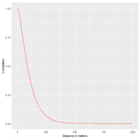
Using a handy function from Greg Albery we can derive the predicted correlation between two points given there distance:
# devtools::install_github("https://github.com/gfalbery/ggregplot")
library(ggregplot)
library(dplyr)

INLARange(ModelList = m_inla, MaxRange = 1000, MeshList = mesh, WNames = "i") +
  labs(x = "Distance in meters") +
  theme(legend.position = "none")
Copy
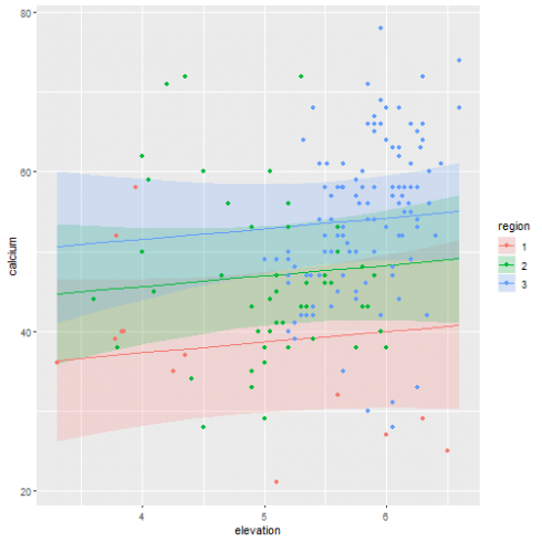
And now we can look at the model predictions first from the fixed effects only, so averaging over the spatial variations:
## first we create an index to easily find these
## prediction within the fitted model
id_fixef <- inla.stack.index(all_stack, "prd_fixef")$data

## add to modmat the prediction and their sd
modmat$calcium <- m_inla$summary.fitted.values[id_fixef, "mean"]
modmat$sd <- m_inla$summary.fitted.values[id_fixef, "sd"]

## a plot with the original data
ggplot(dat, aes(x = elevation, y = calcium)) +
  geom_ribbon(data = modmat, aes(ymin = calcium - 2 * sd,
                                 ymax = calcium + 2 * sd,
                                 fill = region),
              alpha = 0.2) +
  geom_line(data = modmat, aes(color = region)) +
  geom_point(aes(color = region))
Copy
Using the tag we defined earlier we can easily grab the relevant lines in the model object that are stored within the summary.fitted.values data frame in the object. There we get the mean and the standard deviation that we then plot together with the original data.
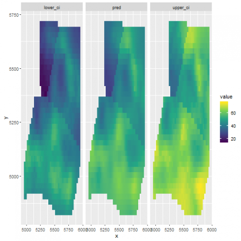
And now come the cool map:
# again get the correct indices
id_alleff <- inla.stack.index(all_stack, "prd_alleff")$data

# now add the model predictions
newdat$pred <- m_inla$summary.fitted.values[id_alleff, "mean"]
newdat$sd <- m_inla$summary.fitted.values[id_alleff, "sd"]
# get lower and upper confidence interval
newdat$lower_ci <- with(newdat, pred - 2 * sd)
newdat$upper_ci <- with(newdat, pred + 2 * sd)

# some data wraggling
nn <- pivot_longer(newdat, cols = c("pred", "lower_ci", "upper_ci"))

ggplot(nn, aes(x=x, y=y, fill=value)) +
  geom_raster() +
  facet_wrap(~name) +
  scale_fill_continuous(type = "viridis")
Copy
There we see one of the advantage of Bayesian analysis, we can get estimation of variation and uncertainty around any estimated quantities from the model.
Voila! That's all for today, next time we will continue along the Bayesian lines with Gaussian Process in greta, get excited!
Some handy refenrences for further reading:
- A couple of pretty handy and very deep tutorials on INLA (not just spatial models): flutterbys.com.au
- The official website: r-inla.org
- Another tutorial for : lattice spatial data


