In the first part I created the data for testing the Astronomical/Astrological Hypotheses. In this part, I started by fitting a simple linear regression model.
mod.lm = lm(div.a.ts~vulcan.ts)
summary(mod.lm)
Call:
lm(formula = div.a.ts ~ vulcan.ts)

Residuals:
    Min      1Q  Median      3Q     Max
-159.30  -53.88  -10.37   53.48  194.05

Coefficients:
             Estimate Std. Error t value Pr(>|t|)
(Intercept) 621.23955   20.24209  30.690   <2e-16 ***
vulcan.ts     0.06049    0.05440   1.112    0.273
---
Signif. codes:  0 ‘***’ 0.001 ‘**’ 0.01 ‘*’ 0.05 ‘.’ 0.1 ‘ ’ 1

Residual standard error: 77.91 on 38 degrees of freedom
Multiple R-squared:  0.03151,	Adjusted R-squared:  0.006026
F-statistic: 1.236 on 1 and 38 DF,  p-value: 0.2731
Clearly, there is little reason to think that the jump points are related to the adjusted divorce counts given the simple regression model. However, since the data is time series data, there is a possibility that the errors are autocorrelated.
The Box-Jenkins Approach
Following the Box-Jenkins approach to fitting time series, I decided to start by looking at the residuals from the adjusted divorce count model as a stationary time series. I generated two plots; a plot of the correlations between present and lagged variables using the R function acf() and a plot of the partial correlations between present and lagged variables using the R function pacf(). For the autocorrelation and the partial autocorrelation plots the blue lines represent the 95% level.
acf(mod.lm$residuals,
main="autocorrelation of the residuals fitting divorce counts on Ceres, Juno, Vesta, and Pallas breaks")

pacf(mod.lm$residuals,
main="partial autocorrelation of the residuals
fitting divorce counts on Ceres, Juno, Vesta, and Pallas breaks
")
Here there are the plot: First the auto-correlations and next the partial auto-correlations.
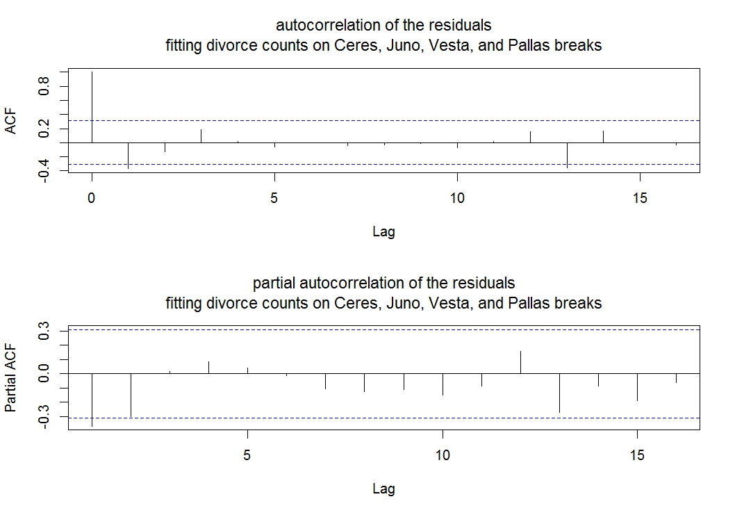
Following the Box-Jenkins approach, the correlation plot will indicate if the time series is a moving average. If there are spikes in the correlation plot, the spikes indicate the orders of the moving average. An autoregressive time series will have an exponentially decaying correlation plot.
The partial correlation plot indicates the order of the process if the process is autoregressive. The order of the auto regressive process is given by the value of the lag just before the partial correlation goes to essentially zero.
A process with both moving average and auto regressive terms is hard to identify using correlation and partial correlation plots, but the process is indicated by decay that is not exponential, but starts after a few lags (see the Wikipedia page Box-Jenkins).
Looking at the above plots, the autocorrelation plot shows negative spikes at lag 1 and lag 13 and is large in absolute value at lags 3, 12, and 14, but otherwise is consistent with random noise. The partial correlation plot has negative spikes at lags 1, 2, and 13 and is large in absolute value at lag 15, indicating that the process may not be stationary. Neither plot decays.
The Periodogram and Normalized Cumulative Periodogram
Using periodograms is another way you can evaluate autocorrelation. A periodogram can find periodicities in a time series. Below are plots of the periodogram and the normalized cumulative periodogram created using spec.pgram() and cpgram() in R. In the periodogram, there are spikes at about the frequencies .35 and .40 that are quite large. The frequencies correspond to lags of 2.9 and 2.5, somewhat close to the lags of 2 and 3 months found in the correlation plot. The normalized cumulative periodogram shows a departure from random noise at a frequency of around .29, or a lag of around 3.4. The blue lines in the normalized cumulative periodogram plot are the 95% confidence limits for random noise.
Plot the periodogram and cumulative periodogram of the residuals from the model.
spec.pgram(mod.lm$residuals,
main="Residuals from Simple Regression
Raw Periodogram")

cpgram(mod.lm$residuals,
main="Residuals from Simple Regression
Cumulative Periodogram")
First the periodogram and next the cumulative periodogram.

Note also that at the frequency of twenty, corresponding to a lag of two, the periodogram is also high.
Using arima() in R to Compare Models
I used the function arima() in R to fit some autoregressive moving average models with orders up to thirteen, both with and without the astronomical regressor. The best model, using the Aktaike information criteria (see the Wikipedia page Aktaike information criterion), was $$Y{_t}=\beta_{0} + \beta_{1}X_{t} + \theta{_1}\epsilon_{t-1} + \theta{_3} \epsilon_{t-1} + \theta_{13} \epsilon_{t-13} + \epsilon_{t}$$ where Yt is the number of divorces in month t, Xt is the number of days since the last shift in the mean of the celestial longitudes of Ceres, Pallas, Vesta, and Juno over the shortest arc, and εt is the difference between the expected number of divorces and the actual number of divorces for month t.
The estimated coefficients, with the respective standard errors, are given in the table below.
| Coefficient | Standard Error | |
| βhat0 | 624 | 10.5 |
| βhat1 | 0.054 | 0.031 |
| θhat1 | -0.682 | 0.274 |
| θhat3 | 0.386 | 0.180 |
| θhat13 | -0.598 | 0.227 |
The final model was fit using arima(). Below, two models are fit, the final one (with the regressor) and one without the regressor.
In arima(), in the argument fixed, an NA indicates the parameter is fit and a 0 indicates no parameter is fit. In fixed there is a value for every value indicated by the arguments order and xreg, plus the intercept. So in the first model below, there are 13 moving average terms, three of which are fit, and there is an intercept and one regressor term, for 15 values in fixed.
The model with the regressor.
mod.arima.r.1 = arima(div.a.ts,
                 order=c(0,0,13),
                 fixed=c(NA,0,NA,rep(0,9),
                 NA,NA,NA),
                 xreg=vulcan.ts)
mod.arima.r.1
Call:
arima(x = div.a.ts, order = c(0, 0, 13), xreg = vulcan.ts, fixed = c(NA, 0,
    NA, rep(0, 9), NA, NA, NA))

Coefficients:
          ma1  ma2     ma3  ma4  ma5  ma6  ma7  ma8  ma9  ma10  ma11  ma12     ma13  intercept
      -0.6822    0  0.3855    0    0    0    0    0    0     0     0     0  -0.5975   623.7144
s.e.   0.2744    0  0.1799    0    0    0    0    0    0     0     0     0   0.2270    10.4553
      vulcan.ts
         0.0541
s.e.     0.0309

sigma^2 estimated as 2618:  log likelihood = -220.54,  aic = 453.07
The model without the regressor
mod.arima.r.2 = arima(div.a.ts,
                 order=c(0,0,13),
                 fixed=c(NA,0,NA,rep(0,9),
                 NA,NA))
mod.arima.r.2
Call:
arima(x = div.a.ts, order = c(0, 0, 13), fixed = c(NA, 0, NA, rep(0, 9), NA,
    NA))

Coefficients:
          ma1  ma2     ma3  ma4  ma5  ma6  ma7  ma8  ma9  ma10  ma11  ma12     ma13  intercept
      -0.6044    0  0.4800    0    0    0    0    0    0     0     0     0  -0.6596   640.3849
s.e.   0.2025    0  0.1775    0    0    0    0    0    0     0     0     0   0.2266     4.7133

sigma^2 estimated as 2655:  log likelihood = -221.92,  aic = 453.85
The coefficient for the slope of the regression is not at least 1.96 times the size of the standard errors of the coefficient, however, the Aktaike information criteria is the smallest for the models at which I looked. The model without the coefficient is a close contender, with the Aktaike information for the two models being 453.07 and 453.85.
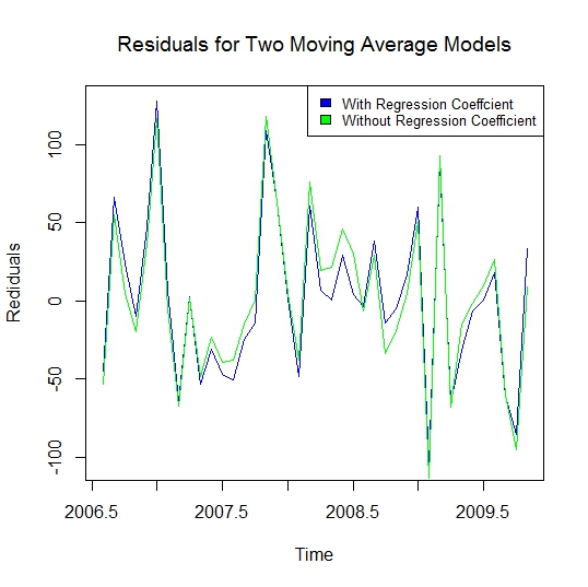
The residuals from the two models are plotted together using ts.plot().
ts.plot(cbind(mod.arima.r.1$residuals,
     mod.arima.r.2$residuals), col=4:3,
     xlab="Time",
     ylab="Residuals",
     main=
     "Residuals for Two Moving Average Models")
legend("topright",
     c("With Regression Coefficient",
     "Without Regression Coefficient"),
     fill=4:3, cex=.7)
Below is a plot of the residuals for the two competing models. To me the residuals look more even for the model given above.
The estimates indicate that the intercept is about 624 divorces; that the number of divorces increases by about 5.4 for every one hundred day increase in the time after the midpoint over the shortest arc of the longitudes of Juno, Ceres, Vesta, and Pallas shifts by 90 or 180 degrees; that errors tend to reverse in direction over one lag and thirteen lags, but tend to be in the same direction over three lags.
Some Concluding Diagnostic Plots
Below are some diagnostic plots; the plot of the residuals versus the fitted values, the Q-Q plot of the residuals versus normal variates, and a time series plot of the actual values and the fitted values.
First the graphic screen is set up to plot three plots in a row. Next the residuals are plotted against the fitted values. Next the residuals are plotted against standard normal percentiles. Last the data is plotted with the fitted values using ts.plot().
par(mfrow=c(1,3))
plot(as.numeric(div.a.ts-
    mod.arima.r.1$residuals),
  as.numeric(mod.arima.r.1$residuals),
  main="Plot of Residuals versus Fitted Values for the Adjusted Divorce Data",
  xlab="Fitted Value",
  ylab="Residual",
  font.main=1)
qqnorm(mod.arima.r.1$residuals,
  main="QQ Normal Plot for Residuals from the Divorce Model",
  font.main=1)
ts.plot(div.a.ts,div.a.ts-
    mod.arima.r.1$residuals,
  ylab="Counts",
  xlab="Year",
  main="Adjusted Divorce Counts and Fitted Counts",
  col=4:3)
legend("bottomleft",
  c("Adjusted Divorce Counts","Fitted Adjusted Divorce Counts"),
  col=4:3, lwd=2, cex=.7)
cor.test(div.a.ts-mod.arima.r.1$residuals,
  mod.arima.r.1$residuals)
Here it is the plot:
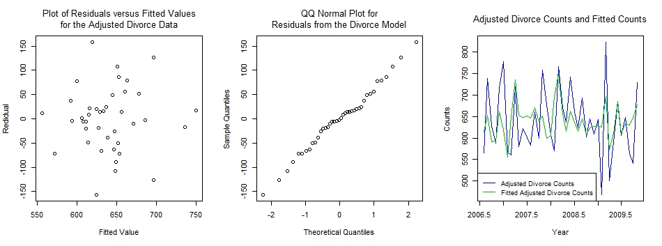
The residual versus fitted value plot looks like there is some correlation between the residuals and the fitted values. Testing the correlation gives a p-value of 0.0112, so the model is not ideal. While the model does not pick up most of the extreme data points, the residual and QQ normal plots do not show any great deviations from a model of normal errors with constant variance. The fitted values were found by subtracting the residuals from the actual data points.
The correlation between the fitted values and the residuals is found and tested for equality with zero using cor.test()
cor.test(div.a.ts-mod.arima.r.1$residuals,
         mod.arima.r.1$residuals)
Pearson's product-moment correlation

data:  div.a.ts - mod.arima.r.1$residuals and mod.arima.r.1$residuals
t = 2.6651, df = 38, p-value = 0.01123
alternative hypothesis: true correlation is not equal to 0
95 percent confidence interval:
 0.09736844 0.63041834
sample estimates:
      cor
0.3968411
The Function to Find the Best Model
Here is the function I created to compare models. The function is set up to only do moving averages. It takes a while to run with ‘or’ equal to 13 for moving averages since 2 to the power of 13, which equals 8,192, arima()’s are run, since each element of fixed can take on either ‘0’ or ‘NA’. If both autoregressive and moving average models are run, then for ‘or’ equal to 13, the function would have to fit 4 to the power of 13 models to get all combinations or 67,108,864 models, which is beyond the capacity of R, at least on my machine.
arima.comp=function(ts=div.a.ts,
phi=vulcan.ts, or=3) {

  phi <- as.matrix(phi)
  if (nrow(phi)==1) phi <- t(phi)
  fx.lst <- list(0:1)
  #for (i in 2:(2*or)) fx.lst <-
  #c(fx.lst,list(0:1))
  for (i in 2:or) fx.lst <-
    c(fx.lst,list(0:1))

  fx.mat <-
    as.matrix(expand.grid(fx.lst))
  #fx.phi1 <- matrix(NA, 2^(2*or),
  #  1+ncol(phi))
  fx.phi1 <- matrix(NA, 2^or,
    1+ncol(phi))

  fx.mat[fx.mat==1] <- NA
  fx.mat1 <-
    cbind(fx.mat,fx.phi1)
  fx.mat2 <-
    cbind(fx.mat,fx.phi1[,1])

  #res1 <- numeric(2^(2*or))
  #res2 <- numeric(2^(2*or))

  res1 <- numeric(2^or)
  res2 <- numeric(2^or)

  #for (i in 1:2^(2*or)) {
  for (i in 1:2^or) {
    #res1[i] <- arima(ts, order=c(or,0,or),
    #  xreg=phi, fixed=fx.mat1[i,])$aic
    #res2[i] <- arima(ts, order=c(or,0,or),
    #  fixed=fx.mat2[i,])$aic

    res1[i] <- arima(ts, order=c(0,0,or),
      xreg=phi, fixed=fx.mat1[i,])$aic
    res2[i] <- arima(ts, order=c(0,0,or),
      fixed=fx.mat2[i,])$aic
  }

  st1 <- order(res1)
  st1 <- st1[1:min(length(st1),10)]
  print(res1[st1])
  print(fx.mat1[st1,])

  st2 <- order(res2)
  st2 <- st2[1:min(length(st2),10)]
  print(res2[st2])
  print(fx.mat2[st2,])
}
In the function, ‘ts’ is the time series to be modeled, ‘phi’ is the vector (matrix) of regressor(s), and ‘or’ is the highest moving average order to be included. To run just autoregressive models, in the calls to arima(), move ‘or’ from the third element of ‘order’ to the first element of ‘order’. In order to run both autoregressive and moving average models, remove the pound signs and add pound signs below where the pound signs were.
In the function, first ‘phi’ is made into a matrix, if a vector. Next the matrices ‘fx.mat1’ and ‘fx.mat2’ are created with the vectors to be assigned to ‘fixed’ in the rows. ‘fx.mat1’ contains regressors and ‘fx.mat2’ does not. Next ‘res1’ and ‘res2’ are created to hold the values of the Aktaike criteria for each model; ‘res1’ for models with a regressor and ‘res2’ for models without a regressor. Next the arima models are fit in a for() loop. Then the numeric order of the elements in ‘res1’ and ‘res2’ are found using order() and only the ten models with the smallest Aktaike criteria are kept, for each of ‘res1’ and ‘res2’. The variables ‘st1’ and ‘st2’ contain the indices of the models with the smallest Aktaike criteria. Last, the values for the ten smallest Aktaike criteria and the values for ‘fixed’ for the ten smallest Aktaike criteria are printed, for models both with and without the regressor.
Some Conclusions
In this part, we have fit a moving average model with a regressor variable to monthly divorce count data from the state of Iowa. The sample size is just 40 observations.
After taking into consideration of the autocorrelations between the observations, we see that divorce counts increase as time passes after a shift in the astronomical point that I call Vulcan – the mean over the shortest arc of the asteroids Juno, Pallas, and Vesta, and the dwarf planet Ceres. The sample size is quite small, so we would not expect a strong effect (highly significant) but the results Indicate that there is some support for the hypothesis that the astronomical point Vulcan is related to divorce counts. Further testing is warranted.
What’s next
In the next part, we use the covariance structure of the model selected in this part to estimate standard errors for differing linear combinations of the monthly counts. The results are interpreted from an astrological point of view.