The assumptions of simple linear regression include the assumption that the errors are independent with constant variance. Fitting a simple regression when the errors are auto-correlated requires techniques from the field of time series. If you are interested in fitting a model to an evenly spaced series where the terms are auto-correlated, I have given below an example of fitting such a model.
The Astronomical/Astrological Hypotheses to be Tested
For some years now, I have been interested in the possible astrological influence of a composite astronomical point, the mean over the shortest arc of the celestial longitudes of the celestial bodies Juno, Ceres, Vesta, and Pallas. I wanted to see if the point affected divorce rates. In astrology, planets rule zodiacal signs. In older systems of astrology, from before the discoveries of the outer planets, each of the five known planets (Mercury, Venus, Mars, Jupiter, and Saturn – we exclude the earth) ruled two signs. As Uranus, Neptune, and Pluto were discovered, the planets were given rulership over one of Saturn’s, Jupiter’s, and Mars’s signs, respectively. In 1977, the celestial body Chiron was discovered. Some astrologers give Chiron the rulership of one of Mercury’s signs, which would leave Venus as the only planet with dual rulership.
The celestial bodies Juno, Ceres, Vesta, and Pallas were discovered in the early 1800’s. Referencing Roman mythology, some astrologers feel that the discoveries of Juno – the wife, Ceres – the mother, Vesta – the sister, and Pallas – the daughter synchronized with the emergence of the struggle for the full participation of women within society. Venus (which, from the above, is for some astrologers the only planet that still rules two signs) is one of the traditional rulers of women in astrology. The two signs that Venus rules are those associated with money and marriage. I had thought that the mean of the celestial longitudes over of the shortest arc connecting Juno, Ceres, Vesta, and Pallas might be the ruler of the sign of marriage, since Juno, Ceres, Vesta, and Pallas refer to female archetypes. Then Venus would just rule the sign of money. The mean over the shortest arc jumps 90 degrees or 180 degrees from time to time. To test the hypothesis, I had thought that the jump point of the mean over the shortest arc might be related to divorce. An ephemeris for the average, which I call Vulcan – as well as a point I call Cent, from 1900 to 2050, can be found here – here.
The Data Sets: Divorce Counts for Iowa and the Jump Points
I created a data vector of monthly divorce counts in Iowa from August of 2006 to November of 2009 and a vector based on the jump points of the mean over the shortest arc of the celestial longitudes of Juno, Vesta, Ceres, and Pallas. The divorce counts were adjusted for the number of business days in a month. The adjusted divorce counts are the dependent variable. The independent variables are the usual column of ones to fit a mean and a column which linearly increases as time increases after a jump point and which is set back to zero at each jump point.
First enter monthly divorce counts for Iowa from 8/06 to 11/09
div.ts = ts(c(619, 704, 660, 533, 683, 778, 541,
         587, 720, 609, 622, 602, 639, 599, 657,
         687, 646, 608, 571, 768, 703, 638, 743,
         693, 624, 694, 660, 522, 639, 613, 446,
         863, 524, 564, 716, 635, 649, 565, 567,
         626), start=c(2006,8), freq=12)
Next enter the break point information: the number of days from the last shift
vulcan.ts = ts(c(63, 94, 124, 155, 185, 216, 247,
            275, 306, 336, 367, 397, 428, 459, 489,
            520, 550, 581, 612, 641, 672, 702, 733,
            763, 19, 50, 80, 4, 34, 65, 96, 124,
            155, 185, 216, 246, 277, 308, 3,  34),
            start=c(2006,8), freq=12)
The divorce data is from the Center for Disease Control and Prevention website, from the National Vital Statistics Report page. I took marriage and divorce data for Iowa from the reports from August of 2006 to November of 2009. The divorce data for April of 2008 was 161, which was unusually small. In my analyses, I replaced the number with 703, the average of the numbers on either side.
The average of the longitudes of the four major asteroids, Juno, Ceres, Pallas, and Vesta (yes, I know Ceres is now a dwarf planet) along the shortest arc will jump by 90 or 180 degrees from time to time. The variable I use is the time in days from the last day in which a jump occurred. Since the marriage and divorce data is monthly, each data point is assumed to be at the 15th of the month.
The question of interest is, are the jump points associated the divorce counts in a linear way? Since the months are not of equal length, I have adjusted the divorce counts by dividing the divorce count for a month by the number of state business days in the month and multiplying the result by the average number of state business days in a month over the observed months.
First create a vector of days of the week, with 1 for Sunday, 2 for Monday, etc. 8/06 started on a Tuesday.
wks = c(3:7, rep(1:7, 173), 1:2)
Next create a daily vector for the months, with 1 for for the first month, 2 for the second month, etc.
mns = c(8:12, rep(1:12,2), 1:11)
mns.d = 1:40
mn =  c(31,28,31,30,31,30,31,31,30,31,30,31)
mns.dys = rep(mns.d,mn[mns])
Add 2008 leap day
mns.dys = c(mns.dys[1:553], 19, mns.dys[554:1217])
Next remove Sundays and Saturdays
mns.dys.r = mns.dys[wks>1 & wks<7]
Next use table() to count the weekdays in each month
mns.dys.s = c(table(mns.dys.r))
Next enter the number of government holidays in each of the 40 months
hol = c(0, 1, 0, 3, 1, 2, 0, 0, 0, 1, 0, 1,
        0, 1, 0, 3, 1, 2, 0, 0, 0, 1, 0, 1,
        0, 1, 0, 3, 1, 2, 0, 0, 0, 1, 0, 1,
        0, 1, 0, 3)
Next subtract out the holidays
mns.dys.s = mns.dys.s - hol
Next adjust the divorce counts
div.a.ts = div.ts * mean(mns.dys.s)/mns.dys.s
The holidays I excluded are New Year’s Day, Martin Luther King Day, Memorial Day, Independence Day, Labor Day, Veteran’s Day, the two days for Thanksgiving, and Christmas Day, as these days were state holidays in Iowa in 2012.
The number of state business days that I found for each month are given in the table below.
| Jan | Feb | Mar | Apr | May | Jun | Jul | Aug | Sep | Oct | Nov | Dec | |
| 2006 | 23 | 20 | 22 | 19 | 20 | |||||||
| 2007 | 21 | 20 | 22 | 21 | 22 | 21 | 21 | 23 | 19 | 23 | 19 | 20 |
| 2008 | 21 | 21 | 21 | 22 | 21 | 21 | 22 | 21 | 21 | 23 | 17 | 22 |
| 2009 | 20 | 20 | 22 | 22 | 20 | 22 | 22 | 21 | 21 | 22 | 18 |
There are 1218 days in the 40 months. The divorce counts are adjusted to reflect the number of days that the county offices are open.
Plotting the Data Sets
Since the dependent variable is a time series, one could expect autocorrelation in the error terms which may need to be taken into account. Below, I have plotted the adjusted divorce counts and the jump point variable.
Next plot the two data vectors:
data.d.v = cbind(
"jump point variable"=vulcan.ts,
"adjusted divorce count"=div.a.ts)
plot(data.d.v, main="
Adjusted Divorce Counts in Iowa with the Jump Point Variable
August 2006 to November 2009")
Here is the plot:
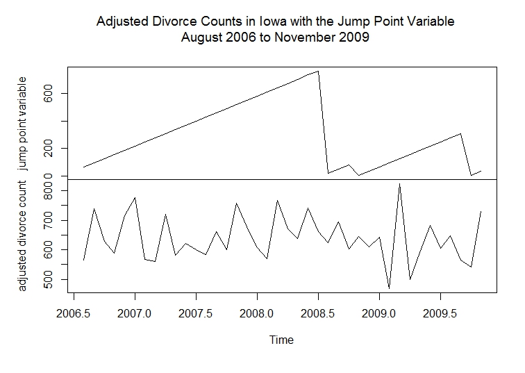
A relationship between the two plots is not immediately evident. Therefore, in the second part we will evaluate the associations by fitting a regression model.