In today’s lesson we’ll continue to learn about linear mixed effects models (LMEM), which give us the power to account for multiple types of effects in a single model. This is Part 2 of a two part lesson. I’ll be taking for granted that you’ve completed Lesson 6, Part 1, so if you haven’t done that yet be sure to go back and do it. The other lessons can be found in there: Lesson 0; Lesson 1; Lesson 2; Lesson 3; Lesson 4; Lesson 5
By the end of this lesson you will:
- Learn about other methods for LMEMs.
- Update our LMEMs in R.
- Summarise the results in an R Markdown document.
We’ll be working off of the same directory as in Part 1, just adding new scripts. There is a video in end of this post which provides the background on the additional math of LMEM and reintroduces the data set we’ll be using today. There is also some extra explanation of some of the new code we’ll be writing. For all of the coding please see the text below. A PDF of the slides can be downloaded here. All of the data and completed code for the lesson can be found here.
Lab Problem
Unlike past lessons where our data came from some outside source, today we’ll be looking at data collected from people who actually took this course. Participants did an online version of the Stroop task. In the experiment, participants are presented color words (e.g. “red”, “yellow”) where the color of the ink either matches the word (e.g. “red” written in red ink) or doesn’t match the word (e.g. “red” written in yellow ink). Participants have to press a key to say what the color of the ink is, NOT what the text of the word is. Participants are generally slower and less accurate when the there is a mismatch (incongruent trial) than when there is a match (congruent trial). Furthermore, we’re going to see how this effect may change throughout the course of the experiment. Our research questions are below.
- Congruency: Are responses to incongruent trials less accurate and slower than to congruent trials?
- Experiment half: Are responses more accurate and faster in the second half of the experiment than the first half of the experiment?
- Congruency x Experiment half: Is there an interaction between these variables?
Setting up Your Work Space
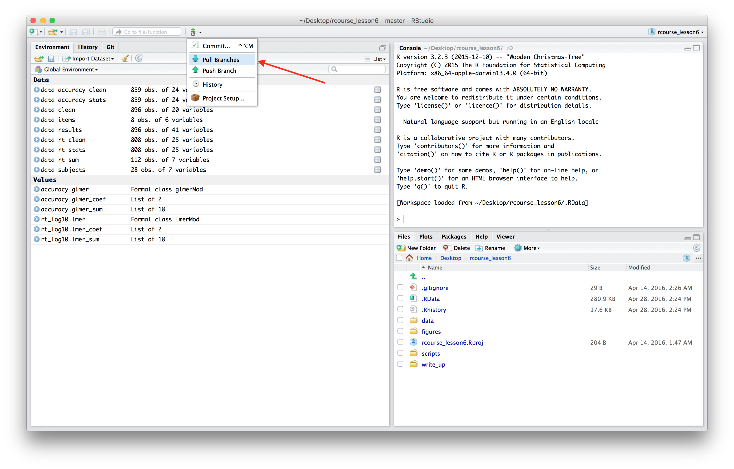
You should already have your workspace setup from Lesson 6, Part 1. Go back into the project from the first part of the lesson. Before beginning the new script go to the “Git” icon and click the “Pull Branches” button. An example screen shot pointing to the button is provided below.
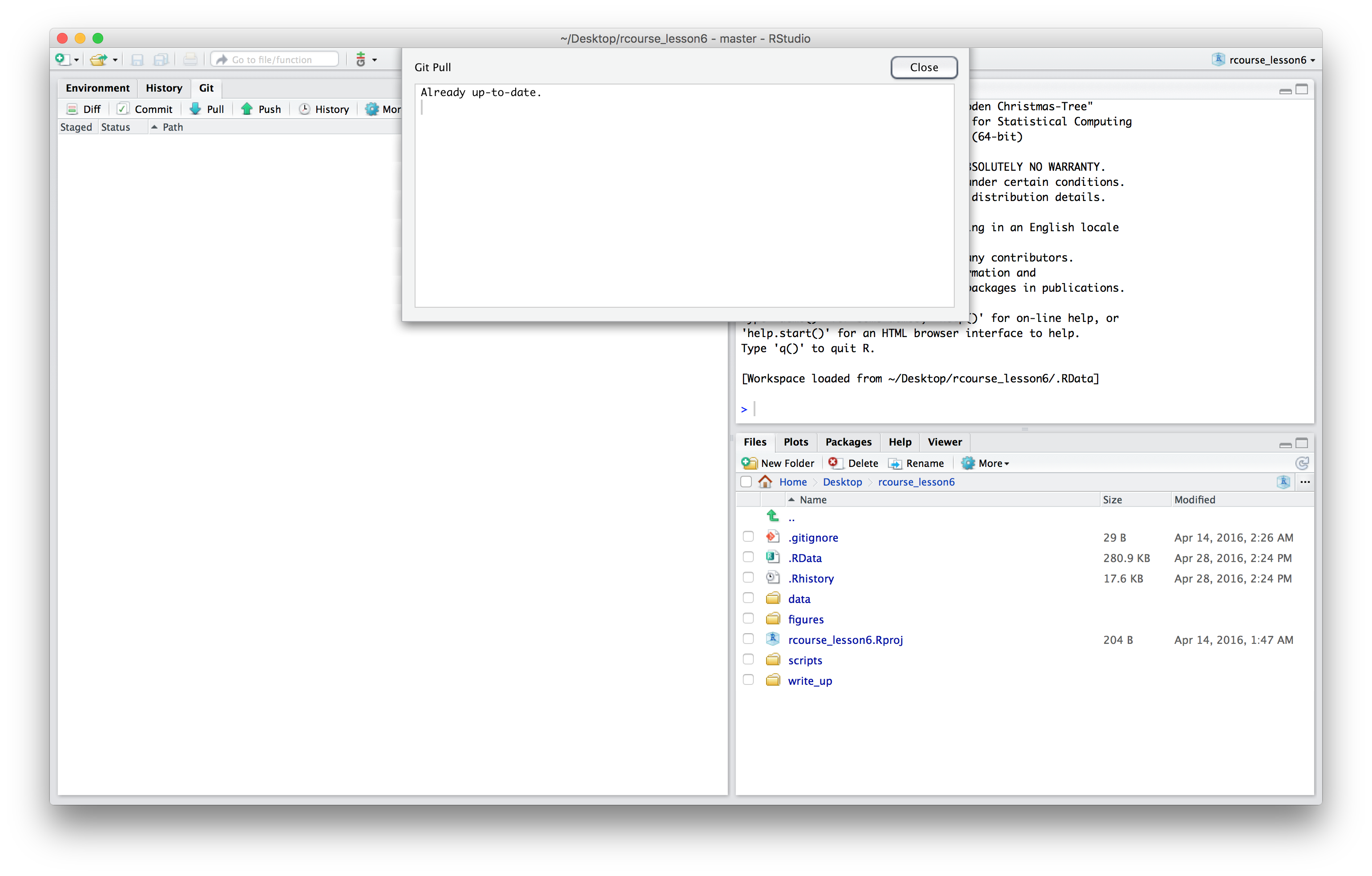
You should get a message saying “Already up-to-date.” (see below for an example). This button pulls down any updates to the repository that are not currently on your computer. Now, since you’re the only one pushing to this repository there shouldn’t have been any updates, thus “Already up-to-date”. However, if you’re working on a project with other people and they all have access to the Bitbucket repository, they may have committed changes in between the times you worked on it, and you want to be sure to pull down those changes before continuing any work. Even though that’s not the case with a repository like this where you’re the only person with access, it’s good to get into the habit of pulling every time you come back to a project for any future projects that you collaborate on with other people.
Now that you’re all up to date we can start scripting again.
Statistics Script (Part 2)
Open a new script and on the first few lines write the following, same as for first statistics script. Note, the results of the models reported in this lesson are based on version 1.1.12 of lme4.
## READ IN DATA ####
source("scripts/rcourse_lesson6_cleaning.R")

## LOAD PACKAGES ####
library(lme4)
We’ll also make our usual header for organizing our data. As for the first statistics script, let’s start with the accuracy data. Unlike in our first script though, now we’re going to add a couple new columns to make our contrast coded variables. Basically for each variable I’m setting one level to “-0.5” and one to “0.5”, so now “0” is directly in between the two levels, but the difference is still “1”. For more details on the code watch the video. In other tutorials you may see that people use the contrasts() call to change data to contrast coding. This also works fine and will produce the same results, I just prefer this method, but do whatever you feel most comfortable with. When you’re ready copy and run the code below.
## ORGANIZE DATA ####
# Accuracy data
data_accuracy_stats = data_accuracy_clean %>%
                      mutate(congruency_contrast = ifelse(congruency == "con", -0.5, 0.5)) %>%
                      mutate(half_contrast = ifelse(half == "first", -0.5, 0.5))
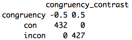
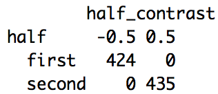
We can also double check that our contrast coding worked appropriately with an xtabs() call. Below are two xtabs() calls with our original columns and our new contrast coded columns.
xtabs(~congruency+congruency_contrast, data_accuracy_stats)
xtabs(~half+half_contrast, data_accuracy_stats)
Below are the outputs of the two calls. As expected for the variable “congruency”, “con” is to “-0.5” and “incon” to “0.5”, and for the variable “half”, “first” is set to “-0.5” and “second” to “0.5”. In the script on GitHub I’ve also included some more calls to double check the random effects structure, but we won’t go over them here since it is the same as in the first statistics script, just changing to our new contrast coded variables.
Now that our variables are contrast coded we can build the new model. Again we’ll start with a model with the maximal random effects structure. The model is the same as our model from the previous lesson except the names of the variables are updated to our contrast coded ones for both the fixed effects and as slopes in the random effects. Copy and run the code below.
## BUILD MODELS FOR ACCURACY ANALYSIS ####
# Full model
accuracy.glmer = glmer(accuracy ~ congruency_contrast * half_contrast +
                                (1+congruency_contrast*half_contrast|subject_id) +
                                (1+half_contrast|item), family = "binomial",
                                data = data_accuracy_stats)
Once again the model did not converge with the maximal random effects structure, matching our model from before. Copy and run the code below.
accuracy.glmer = glmer(accuracy ~ congruency_contrast * half_contrast +
                                  (1|subject_id) +
                                  (0+half_contrast|subject_id) +
                                  (1|item), family = "binomial",
                                  data = data_accuracy_stats)
Again we’ll use the summary() call to get more information about the model. Copy and run the code below.
# Summarise model and save
accuracy.glmer_sum = summary(accuracy.glmer)
accuracy.glmer_sum
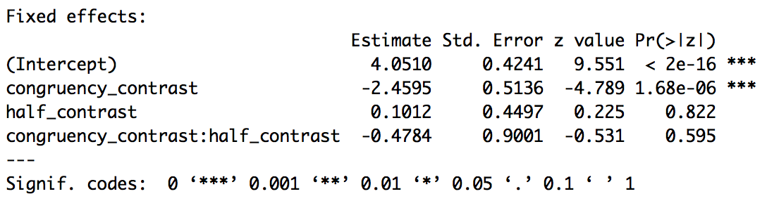
Part of the output of the summary call is below. Now that we’ve contrast coded our variables we can interpret the results as we would an ANOVA. The intercept is now the grand mean of the data (in logit space) given our random effects. The effect of congruency tells us that subjects are less accurate on incongruent trials (since incongruent is the positive value and the estimate is negative), but now we can say this across the whole experiment, not just within the first half of the experiment. There continues to be no effect of experiment half and no interaction.
I won’t go over the code for looking at the random effects coefficients, but the code is in the script on GitHub. Instead of trusting the p-values from the z-scores though, we’re going to use model comparison. Next we can test for our first variable, congruency. To do this we’ll build the same model but subtracting “congruency_half”. Copy and run the code below.
# Test for effect of congruency
accuracy_congruency.glmer = glmer(accuracy ~ congruency_contrast * half_contrast -
                                                    congruency_contrast +
                                             (1|subject_id) +
                                             (0+half_contrast|subject_id) +
                                             (1|item), family = "binomial",
                                             data = data_accuracy_stats)
With our model built we can make and view the comparison between the original full model and the model without congruency. Copy and run the code below.
accuracy_congruency.anova = anova(accuracy.glmer, accuracy_congruency.glmer)
accuracy_congruency.anova
Below is the output of the anova() call (which is really a likelihood ratio test). As you can see the AIC for the reduced model (“accuracy_congruency.glmer”) is larger than for the full model (“accuracy.glmer”) suggesting that including congruency does significantly improve the fit of the model (remember, lower AIC is better). Indeed this is confirmed by the likelihood ratio test that finds a significant difference between the two models (with significance set at p < 0.05). So, as expected there is a significant effect of congruency.
![]()
Let’s do the same thing now for the variable experiment half. Below is the full code block making the new model and the anova() call to compare to the original full model.
# Test for effect of experiment half
accuracy_half.glmer = glmer(accuracy ~ congruency_contrast * half_contrast -
                                              half_contrast +
                                       (1|subject_id) +
                                       (0+half_contrast|subject_id) +
                                       (1|item), family = "binomial",
                                       data = data_accuracy_stats)

accuracy_half.anova = anova(accuracy.glmer, accuracy_half.glmer)
accuracy_half.anova
Below is the output of the model comparison. This time the reduced model (“accuacy_half.glmer”) has a lower AIC than the full model, but this difference is not significant, so including (or excluding) experiment half does not significantly improve the model.
![]()
Our final model subtracts the interaction of congruency and experiment half. Remember that the * symbol includes both the main effects and the interaction, to only subtract the interaction we use :. Copy and run the code below.
# Test for interaction of congruency x experiment half
accuracy_congruencyxhalf.glmer = glmer(accuracy ~ congruency_contrast * half_contrast -
                                                         congruency_contrast:half_contrast +
                                                  (1|subject_id) +
                                                  (0+half_contrast|subject_id) +
                                                  (1|item), family = "binomial",
                                                  data = data_accuracy_stats)

accuracy_congruencyxhalf.anova = anova(accuracy.glmer, accuracy_congruencyxhalf.glmer)
accuracy_congruencyxhalf.anova
Below is the output of the model comparison. Again the reduced model has a slightly lower AIC, but not significantly so. So, the interaction does not significantly affect the model.
![]()
Overall our results from both the figure and our first LMEM are confirmed. There is an effect of congruency on accuracy, but not experiment half and there is no interaction. Now let’s move on to the reaction time analysis.
Start by going back to the top of the script to the “ORGANIZE DATA” section. Below the xtabs() calls for the accuracy analysis we’re going to make our data frame for the reaction time analysis. We’ll do the same thing we did for the accuracy data by adding two columns contrast coding our independent variables. Copy and run the code below.
# RT data
data_rt_stats = data_rt_clean %>%
                mutate(congruency_contrast = ifelse(congruency == "con", -0.5, 0.5)) %>%
                mutate(half_contrast = ifelse(half == "first", -0.5, 0.5))
As for the accuracy data we can also run a couple xtabs() calls to double check our work. The code is below, but I won’t put the output here. Copy and run the code to double check for yourself though.
xtabs(~congruency+congruency_contrast, data_rt_stats)
xtabs(~half+half_contrast, data_rt_stats)
Now we can start building our model. Below is the code for the model with maximal random effects structure. Like our accuracy model all of the references to our fixed effects are changed to our new contrast coded variables. There is also the addition of the call REML = F. This has to do with how the variance is computed and we need to set it to FALSE for when we later do our model comparison to get our p-values. Copy and run the code below.
## BUILD MODELS FOR REACTION TIME ANALYSIS ####
# Full model
rt_log10.lmer = lmer(rt_log10 ~ congruency_contrast * half_contrast +
                                (1+congruency_contrast*half_contrast|subject_id) +
                                (1+half_contrast|item), REML = F,
                                data = data_rt_stats)
Unlike in the dummy coded model, the model does not converge. However, all we have to do is uncorrelate the random intercept and random slope for “item”. Copy and run the updated code below.
rt_log10.lmer = lmer(rt_log10 ~ congruency_contrast * half_contrast +
                                (1+congruency_contrast*half_contrast|subject_id) +
                                (1|item) +
                                (0+experiment_half|item), REML = F,
                                data = data_rt_stats)
Let’s get the summary of the model and look at it. Copy and run the code below.
rt_log10.lmer_sum = summary(rt_log10.lmer)
rt_log10.lmer_sum
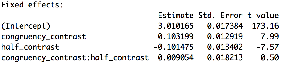
Below is part of the summary output. Remember, we don’t get p-values with lmer() but we can get initial impressions based on the t-values (absolute values greater than 2 likely significant at p < 0.05). Based on these t-values we appear to have an effect of congruency and experiment half, but now we can confidently say this applies to the data as a whole, not just given specific baselines.
To test for the effect of congruency, copy and run the code below.
# Test for effect of congruency
rt_log10_congruency.lmer = lmer(rt_log10 ~ congruency_contrast * half_contrast -
                                       congruency_contrast +
                                (1+congruency_contrast*half_contrast|subject_id) +
                                (1|item) +
                                (0+experiment_half|item), REML = F,
                                data = data_rt_stats)

rt_log10_congruency.anova = anova(rt_log10.lmer, rt_log10_congruency.lmer) rt_log10_congruency.anova
The reduced model has a larger AIC then the full model (yes, 1143.3 is smaller than 1164.0 but they are negative, and -1149.2 is larger than -1169.8). We have this difference statistically confirmed by the likelihood ratio test, so indeed having congruency significantly improves the model.
![]()
Next we can test for the effect of experiment half. Copy and run the code below.
# Test for effect of experiment half
rt_log10_half.lmer = lmer(rt_log10 ~ congruency_contrast * half_contrast -
                                       half_contrast +
                                (1+congruency_contrast*half_contrast|subject_id) +
                                (1|item) +
                                (0+experiment_half|item), REML = F,
                                data = data_rt_stats)

rt_log10_half.anova = anova(rt_log10.lmer, rt_log10_half.lmer)
rt_log10_half.anova
Below is the output of the model comparison. We again get a larger (less negative) AIC for the reduced model. This difference is confirmed to be significant. So, as expected adding experiment half improves the model.
![]()
Finally, below is the code to test the interaction. Copy and run the code below.
# Test for interaction of congruency and experiment half
rt_log10_congruencyxhalf.lmer = lmer(rt_log10 ~ congruency_contrast * half_contrast -
                                       congruency_contrast:half_contrast +
                                (1+congruency_contrast*half_contrast|subject_id) +
                                (1|item) +
                                (0+experiment_half|item), REML = F,
                                data = data_rt_stats)

rt_log10_congruencyxhalf.anova = anova(rt_log10.lmer, rt_log10_congruencyxhalf.lmer)
rt_log10_congruencyxhalf.anova
Below is the model comparison output. As expected, the interaction does not appear to have any effect on the model.
![]()
Overall our initial expectations are confirmed. Subjects are slower on incongruent trials and faster in the second half of the experiment, however there is no interaction of these variables. Across all of the data we get congruency effects for both accuracy and reaction times but experiment half only matters for reaction times, not accuracy.
One quick word to the wise for using this method. I have found random effects structures that converged for the full model but then wouldn’t converge for some of the reduced models. Following the edict that we can’t trust models that don’t converge I then further reduced my original model until all models (the full one and all of the reduced models) converged. This can take a while and be frustrating but it’s better to be sure that all of your models are converging.
You’ve now successfully gotten rid of the baseline issue and used a more robust method for significance testing! Save your script in the “scripts” folder and use a name ending in “_pt2_statistics”, for example mine is called “rcourse_lesson6_pt2_statistics”. Once the file is saved commit the change to Git. My commit message will be “Made part 2 statistics script.”. Finally, push the commit up to Bitbucket.
Write-up
Let’s make our write-up to summarise what we did today. First save your current working environment to a file such as “rcourse_lesson6_environment” to your “write_up” folder. If you forgot how to do this go back to Lesson 1. Open a new R Markdown document and follow the steps to get a new script. As before delete everything below the chuck of script enclosed in the two sets of ---. Then on the first line use the following code to load our environment.
```{r, echo=FALSE}
load("rcourse_lesson6_environment.RData")
```
Let’s make our sections for the write-up. I’m going to have four: 1) Introduction, 2) Methods, 3) Results, and 4) Conclusion. I’ll also have a few subsections. See below for structure.
# Introduction


# Methods

## Participants

## Materials

## Procedure


# Results

## Accuracy

## Reaction Times


# Conclusion
In each of my sections I can write a little bit for any future readers. For example below is my Introduction. You’ll notice that I include the link to Wikipedia article on the Stroop effect.
# Introduction

The [Stroop effect](https://en.wikipedia.org/wiki/Stroop_effect) is a well known example in psychology of when it is difficult to ignore conflicting information. My data comes from participants in an R course who conducted the experiment online.
In my Methods section you’ll see I use a lot of inline R code. This is useful if you add more data later and want to update your report without having to manually recompute information. For example, in the Participants section I specify the number of native and non-native French speakers simply using R code. See below for the example.
## Participants

Participants were `r length(unique(data_subjects$subject_id))` French speakers, some native (`r length(unique(subset(data_subjects, native_french == "yes")$subject_id))`) and some non-native (`r length(unique(subset(data_subjects, native_french == "no")$subject_id))`) French speakers. There were `r length(unique(subset(data_subjects, sex == "female")$subject_id))` females and `r length(unique(subset(data_subjects, sex == "male")$subject_id))` males. The average age of all participants was `r round(mean(data_subjects$age), 2)` years old.
Moving to the Results section, I again use a lot of inline R code to present the results of the analysis. Below is an example from the accuracy analysis.
The model found a significant effect of congruency, such that there was lower accuracy on incongruent trials compared to congruent trial [$\beta$ = `r round(coef(accuracy.glmer_sum)[2,1], 2)`, *SE* = `r round(coef(accuracy.glmer_sum)[2,2], 2)`, $\chi^2$(1) = `r round(accuracy_congruency.anova$Chisq[2], 2)`, *p* $<$ 0.05]. There was no effect of experiment half and no significant interaction of congruency and experiment half.
Go ahead and fill out the rest of the document to include the full results and a conclusion, you can also look at the full version of my write-up with the link provided at the top of the lesson. When you are ready, save the script to your “write_up” folder (for example, my file is called “rcourse_lesson6_writeup”) and compile the HTML or PDF file. Once your write-up is made, commit the changes to Git. My commit message will be “Made write-up.”. Finally, push the commit up to Bitbucket. If you are done with the lesson you can go to your Projects menu and click “Close Project”.
Congrats! You can now do an LMEM with contrast coding and get p-values with model comparison in R!
Conclusion and Next Steps (Beyond this Course)
Today you continued learning about LMEMs by using contrast coding and model comparison, thus taking care of our baseline issues in a model with an interaction without having to run an ANOVA. You also extended your use of inline R code in an R Markdown document. This lesson marks the end of the course R for Publication. I hope you found the course useful and will be able to use what you learned here in future R programming!