Before starting this lesson you should have completed all of the steps in Lesson 0. If you have not, go back and do the lesson now. The other lessons can be found in there: Lesson 2; Lesson 3; Lesson 4; Lesson 5; Lesson 6, Part 1; Lesson 6, Part 2.
By the end of this lesson you will be able to:
- Make an R Project.
- Commit to Git.
- Push to Bitbucket.
- Read in and manipulate data.
- Make a figure and save it to PDF.
- Create an R Markdown document.
Introduction
There is a video in end of this post which provides an overview of the lesson and some more detailed explanation of the R code we’ll write below. A PDF of the slides can be downloaded here. Before beginning please download this text file, it is the data we will use for the lesson. We’ll be using some fake picture naming reaction time data from bilinguals and monolinguals. All of the data and completed code for the lesson can be found here.
Make an R Project
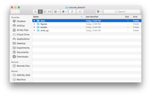
An R Project is a powerful way to have a self-contained environment for each of your projects. Using Projects also allows us to commit to Git which is a useful method of version control. Before we make a Project though we’re going to start by making our directory that will store everything we’re going to do in RStudio. I’m going to create a folder called “rcourse_lesson1” and then inside of it four folders: 1) “data”, 2) “figures”, 3) “scripts”, and 4) “write_up”. See the example folder below.
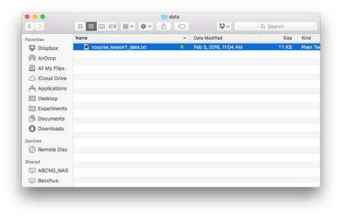
I’m also going to put my data file (“rcourse_lesson1_data.txt”) into my “data” folder so that it looks like below.
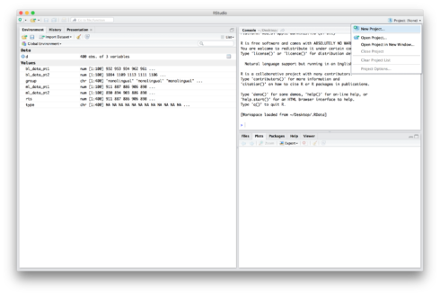
Okay, we’re now ready to make a Project. To make a new Project, go to the top right hand corner of RStudio and click on where it says “Project: (None)” and then choose “New Project…”. An example screen shot is provided below. I want to quickly note that your RStudio may not look exactly the same as mine. For example, you may have the console in the bottom left hand corner instead of the top right. If you want to change the arrangement of your panes go to “Preferences” → “Pane Layout”.
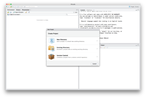
You will be asked if you want to save the current workspace. If you have something important there click “Save”, if you’re not sure click “Save”, otherwise feel free to click “Don’t Save”. A window will then popup asking you how you would like to create your project: 1) “New Directory”, 2) “Existing Directory”, or 3) “Version Control”. See below for an example of what the window should look like.
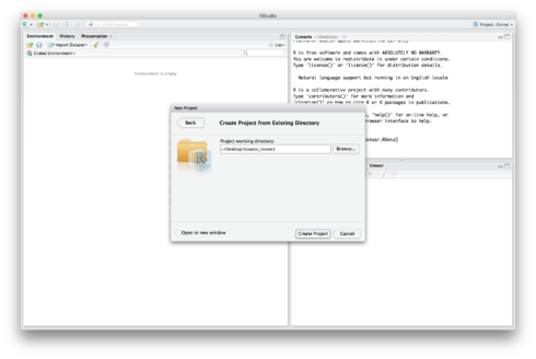
Since we just created our folder structure choose “Existing Directory”. Then use the “Browse…” button to find our root folder. The file path to mine is “~/Desktop/rcourse_lesson1”, as displayed below, since I created my folders on the Desktop. Note, DO NOT browse into one of the sub folders we created (e.g. “data”), be sure to only browse into the main root directory.
When you’ve navigated to your folder click “Create Project”. You’ve just successfully created a R Project!
Commit to Git
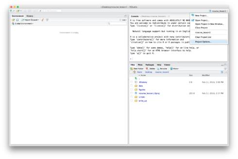
Before beginning any coding we’ll want to make sure that our version control (Git) is set up. To do this go to the top right hand corner that you went to originally to make your project. It should now say the name of your project (for example, mine says “rcourse_lesson1”). Click on it and then choose “Project Options…” as shown below.
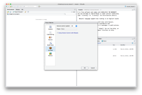
A window will pop up called “Project Options”. On the left hand side menu choose “Git/SVN” and change the setting of “Version control system” from “(None)” to “Git”. A message will then pop up asking you if you confirm the Git repository, say “Yes”. You will also get a message asking if it is okay to restart RStudio, say “Yes”. You should now see the word “Git” on its side in grey, red, and green in the top menu bar. If you navigate back to the “Git/SVN” page of the “Project Option” it should say “Git”. An example screen shot of the “Project Options” window after you’ve set “Version control system” to “Git” is below.
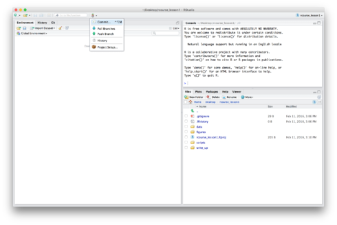
Now that we have Git enabled for our project we should actually commit something. We don’t have much to commit seeing as we have no scripts or figures, but we do have our initial folder structure and the data. To commit to Git click on the sideways “Git” in the menu bar and choose “Commit…”. An example is given below.
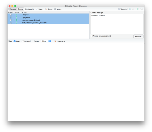
This should give you a pop up window that lists everything new that hasn’t been committed to Git yet. To commit something either click the box under “Staged” or select an item and then click “Stage” in the top menu. Select everything so that all boxes are checked (as shown below). Finally, write a message in the window for “Commit message”. Generally for my first commit I just write “Initial commit.” as is done below. When you’re ready click “Commit”.
You will now see a window that summarizes all of the changes committed to Git, click “Close”. You should notice that the box that previously listed our files is now empty, that’s because you have nothing new to commit. You can now close this window. Good job, you’ve just done your first Git commit!
Push to Bitbucket
In addition to committing locally on our personal computer, we’re also going to be pushing our R code up to Bitbucket. When you’re committing to Bitbucket for the first time there are a few steps you need to do. After your first commit though everything will be done directly in RStudio.
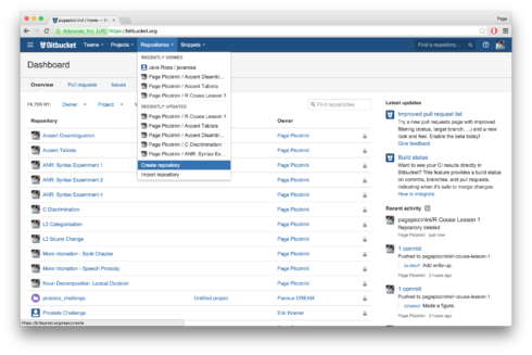
Logon to Bitbucket and on the top menu bar choose “Repositories” and then “Create repository”. See example below.
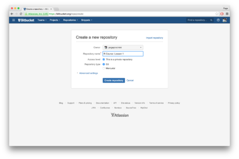
On the following page type in the name of your repository in “Repository name”, I chose “R Course: Lesson 1”. Leave everything else as is and click “Create repository”.
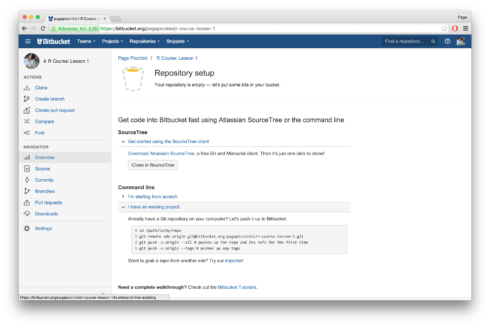
You should now be on a page like the one below. Under the section for “Command line” click on “I have an existing project”, as we do indeed already have a directory and one initial Git commit. You should see some Terminal code in the box under “Already have a Git repository on your computer? Let’s push it to Bitbucket.” We’ll go through each line now.
The first line of the Terminal code
cd /path/to/my/repoCopy
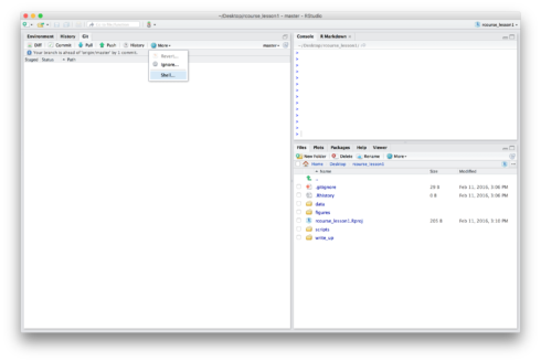
is simply telling you to navigate to your root folder we created earlier. If you are on a Unix-like machine open the Terminal and navigate to the root folder (for me it’s “rcourse_lesson1”). If you are on a Windows machine right click on the folder and choose “Git Bash Here”. Another option is to open the Terminal directly from RStudio, go to the “Git” tab, then “More”, and then choose “Shell…”. This will open a Terminal window already in the folder of your project. This should work fine for Unix-like machines but may be less reliable for Windows machines.
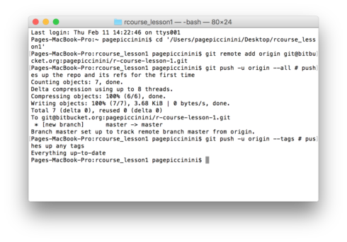
Once you have navigated to the correct folder copy and paste the second line of the code from Bitbucket into the terminal. Remember, the line below is specific to me and my Bitbucket account. Be sure to copy and paste the code that you see in your browser.
git remote add origin git@bitbucket.org:pagepiccinini/r-course-lesson-1.gitCopy
The code should run very quickly and you won’t produce an kind of messages. Now copy and paste the third line of code. If this is your first time pushing to Bitbucket you will be asked if you can accept their SSH RSA key, say yes. Also, if you created a passphrase you’ll have to type it in now.
git push -u origin --all # pushes up the repo and its refs for the first timeCopy
This may take a little bit of time depending on your internet connection, you should be given updates about how far into the upload you are. Finally, copy and paste the last line of code.
git push -u origin --tags # pushes up any tagsCopy
If everything ran correctly after this line you should get a message that says “Everything up-to-date”. An example Mac Terminal is provided below.
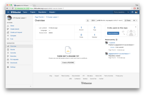
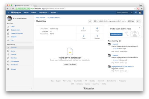
You’ve now successfully uploaded your R Project to Bitbucket! To confirm this go back to Bitbucket and refresh the page. The instructions for uploading should now be replaced with a summary of the repository and a history of your past commits on the right hand side. An example screen shot is provided below.
Read in and Manipulate Data
Now that Git is set up both locally for the project and with Bitbucket we can finally start coding in R. In RStudio go to “File”→ “New File”→ “R Script”. The first thing we’re going to do is read in our data, but even before that we’re going to get ready to read in our data by loading packages. In R the # symbol is used for comments. I generally start all of my code with a comment about loading packages and then load any packages that I need. For this lesson we’ll be using both dplyr and ggplot2 Also, if you end a line with four #s it is a code block, and can be collapsed using the small black arrow if you want to only look at a certain part of your code. Start your script by writing and running the code below. To run a particular line of code from a script make sure the cursor is on the line of code you want to run and press Command+Enter on a Mac or Ctrl+Enter on a Linux or Windows machine. To run several lines of code, highlight all the lines you want to run and then press Command+Enter or Ctrl+Enter. You can also click the “Run” button in the top right hand corner of the script. Remember, all of the code fully commented can be found at the link at the top of the lesson.
## LOAD PACKAGES ####
library(dplyr)
library(ggplot2)Copy
We can now read in our data. Again I’ll start with a section header comment to note what I’ll be doing in this section and then a sub comment with more specific information about this call. Write the following code and then run it.
## READ IN DATA AND ORGANIZE ####
# Read in data
data = read.table("data/rcourse_lesson1_data.txt", header = T, sep = "\t")Copy
To read in data we use the read.table() call. For R Projects the working directory is always set to the root folder, so in order to load our data into R we need to first go into the “data” folder and then call the text file, thus our call is “data/rcourse_lesson1_data.txt”. The header = T part of the code let’s R know that the first row of our file includes our variable names, so it should be treated as a header not as a row of data. Finally the sep command is used to tell R what format the data is in. This is a tab delineated file so we set sep to "\t".
Now that we have the data loaded we can look at it. Below are some calls to examine our data such as dim() (which tells us the number of rows and columns), head() (which prints the first six rows), and tail() (which prints the last six rows). I’ve also included an xtabs() call, which is a way to see how many data points are in a given level of a variable. For example, the call here sees how many data points we have in the two levels of “group”, “bilingual” and “monolingual”. Write and run the code below.
# Look at data
dim(data)
head(data)
tail(data)
xtabs(~group, data)Copy
So far all of this has been basic R code, but now we’re going to use some dplyr code for the first time. Let’s say we want to create a new data frame with only data from our bilinguals. To do this we need to subset out, or filter, “data” to only include bilingual data. We’ll save this to a new data frame called “data_bl”. The code for how to do this is below. For more information on what each part of the code means watch the video or look at the slides at the top of the lesson. Remember, this code will only run if you loaded the dplyr package earlier.
# Subset out bilinguals
data_bl = data %>%
          filter(group == "bilingual")Copy
The main thing that may seem strange to you is the %>% code. This is called a “pipe” in dplyr terminology or an infix operator in more general R terminology. It is a way to letting R know that you’re not done writing code. So, R will not execute the code until it gets a line that doesn’t end in %>%. As a result you can stack several dplyr calls in different lines which gives you cleaner, easier to read code. See the video and slides above for an example of adding another filter() call.
We can now look at our new data frame “data_bl” just like we did for “data”. We can see that it has half as many rows as “data” with dim(). Using xtabs() we also see that there are no data points for “group” “monolingual”, which is good since that was our goal with the filter() call. I’ve also added another xtabs() call on the variable “type”. We see that bilinguals are split into two types, “high” and “low”.
# Look at bilingual data
dim(data_bl)
head(data_bl)
tail(data_bl)
xtabs(~group, data_bl)
xtabs(~type, data_bl)Copy
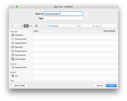
Now that we’ve done a fair amount of coding it’s a good idea to save our script. Be sure to save the script in the “scripts” folder as shown below. Here I named my script “rcourse_lesson1”.
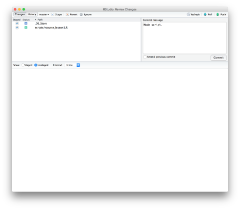
Since we saved our script we’ll also want to commit it to Git. To do this go back to the “Git” menu at the top and choose “Commit…” just like we did for our initial commit. Once again check all of the boxes of changed files and write a message in the “Commit message” window, I wrote “Made script.”. When you are ready click “Commit”.
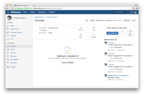
Click “Close” on the message window but don’t close out of the Git window just yet. We’ve committed to Git locally but we haven’t pushed that commit up to Bitbucket. To do that all you have to do is click the button in the top right hand corner that says “Push” with an upwards pointing arrow. You will get a message about the commit. When it is done click “Close” and then close out of the Git window. To confirm that your push to Bitbucket did indeed take place go back to Bitbucket in your browser and refresh the page. You should now see your newest commit with its message in the right hand side of the page as shown below.
See how easy that was! All future commits and pushes can also happen directly within RStudio, letting you have both a local and online record of all of your work.
Make a Figure
We’ve now gotten some experience with dplyr but none yet with ggplot2, specifically making a figure. We’ll start by making a boxplot of reaction times separated by our two groups. To do this type in and run the code below. Again, I’ve started with a section header and then another sub comment about the plot itself.
## MAKE FIGURES ####
# By group
data.plot = ggplot(data, aes(x = group, y = rt)) +
            geom_boxplot()
data.plotCopy
See the video and slides for details of each part of the code. The key features to note are that every plot in ggplot2 is initiated with the call ggplot(). We then give it our data frame and set the aesthetics (aes()). On the second line we say what type of plot we’ll be making, in this case a boxplot. Most ggplot2 specific plots are made with geom_ and then the type of plot to make, in this case boxplot. Also note that for ggplot2, to connect lines of code we use the + operator not the %>% operator. All of this is assigned to “data.plot” and then we call “data.plot” to see the figure.
Right now we only have our plot locally in RStudio. Presumably you’ll want to get a file version of the plot to include in papers or presentations. Below is an updated version of the code to print the plot to a PDF. The first line calls the call pdf(). Note, I want my figure to go into my “figures” folder, so when I give the file path to pdf() I start with figures/ before naming the plot “data.pdf”. I then have my plot call and end with dev.off() to close the graphics device pdf(). If you look in the “figures” folder you should now find a PDF of the figure you saw in RStudio.
## MAKE FIGURES ####
# By group
data.plot = ggplot(data, aes(x = group, y = rt)) +
            geom_boxplot()
pdf("figures/data.pdf")
data.plot
dev.off()Copy
Once again we need to commit our updates to Git and then push to Bitbucket. Go to “Git” in the top menu, “Commit…”, select all modified files, write a commit message (e.g. “Made figure.”), and then click “Commit”. Before closing the window be sure to click “Push” to send it up to Bitbucket. Now when you refresh Bitbucket in your browser you should see your most recent commit.
You have successful made a figure, saved it to a PDF, committed your work to Git, and pushed that commit up to Bitbucket. Congrats!
Create an R Markdown Document
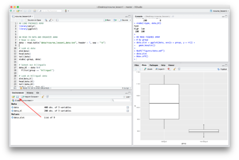
The final thing we’ll be doing today is creating an R Markdown document to showcase all of our amazing work. The first thing we need to do is save our environment, which has our data, our subsetted data, and our figure. To save the environment be sure you are in the “Environment” tab in RStudio, then click on the figure of the floppy disk to save it. See the screen shot below. A red arrow is pointing to where you should see the floppy disk. Remember though, the “Environment” tap may be in a different pane on your screen.
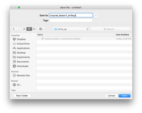
Choose your “write_up” folder for where to save the environment and give it a name like I did below such as “rcourse_lesson1_environment”. Press save when ready.
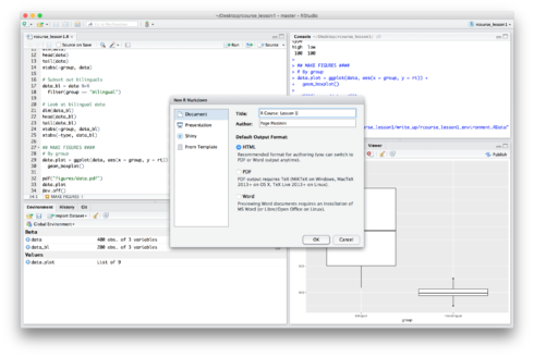
Now with our environment saved we can start writing up our results. To make an R Markdown document go to “File” → “New File” → “R Markdown…”. Either now or in a moment you may be asked to install some packages. These are required to create our documents, agree to any package installs. A window will pop up asking for more information. Make sure “Document” is chosen from the right hand side bar (it should be automatically). In “Title” write whatever you want, I’ve chosen “R Course: Lesson 1”. For “Author” it should be your name by default, if not fill in your name. For “Default Output Format” choose “HTML” if it is not already selected. When you’re ready click “OK”.
The file will by default have some text pre-added that give examples of how to use R Markdown documents. Feel free to read through it, but when you’re ready delete everything below the following code
---
title: 'R Course: Lesson 1'
author: "Page Piccinini"
date: "February 11, 2016"
output: html_document
---Copy
and on the first line below the second set of “—“s type
```{r}
load("rcourse_lesson1_environment.RData")
```Copy
The use of the ```{r} and final ``` let’s RStudio know that this part should be read as R code, not as normal text. Any time you type text not inside those commands it well be printed the same way it would be in text file and not read as code. The load() call tells RStudio to read in that environment file we saved earlier. Note, up until now all file paths have been based on the root directory, so why don’t we write write_up/rcourse_lesson1_environment.RData? It’s because RMarkdown documents are special, and their directory is based on where the R Markdown document itself is saved, so we can just directly type the name of the environment file since it will be in the same folder as our R Markdown document.
On the next line we can start writing up our document. Type in the text below:
# Data
Here is a look at our two data frames. First is the one we read in, the second is our subset of just the bilinguals' data.
# Figure
Here's a figure of the bilinguals compared to the monolinguals.Copy
Note, that this is just regular text, and is not enclosed it our command to be run as R code. Also, while in R scripts the # is used for commenting in Markdown # is used to mark formatting, specifically sections, # is the highest section ## a subsection and so forth.
We’re not going to want to just write about our data and figure though, we’re going to want to actually see them. I’ve updated the code to now include two chunks of R code, the first will display the first few rows of both of our data frames and the second will print our figure. I’ve also added the fig.align='center' call to make sure our figure is centered.
# Data
Here is a look at our two data frames. First is the one we read in, the second is our subset of just the bilinguals' data.
```{r}
head(data)
head(data_bl)
```
# Figure
Here's a figure of the bilinguals compared to the monolinguals.
```{r, fig.align='center'}
data.plot
```Copy
When you have all of this typed into your R Markdown document click the button that says “Knit HTML”. You will be asked to save the R Markdown document before continuing. Navigate to the “write_up” folder, name your file, and save it. See example below.
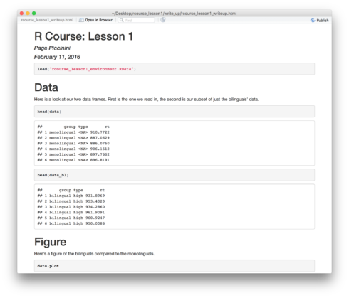
Press “Save” when ready and it will create your document. You show now have a document something like the one below that.
If you want to make a PDF instead of an HTML file simply go back to your R Markdown document and next to where you clicked “Knit HTML” there should be a downward pointing black arrow, click it and choose “Knit PDF”. You can switch back and forth between HTML and PDF as much as you like. Note, if you do not have some kind of Tex installed this will not work. RStudio’s PDF compiler is based on Tex. This should give you a PDF like the one below.
As always we’re going to want to commit these changes to Git and then push up to Bitbucket. Go to “Git” in the top menu, “Commit…”, select all modified files, write a commit message (e.g. “Made write-up.”), and then click “Commit”. Before closing the window be sure to click “Push” to send it up to Bitbucket. Now when you refresh Bitbucket in your browser you should see your most recent commit.
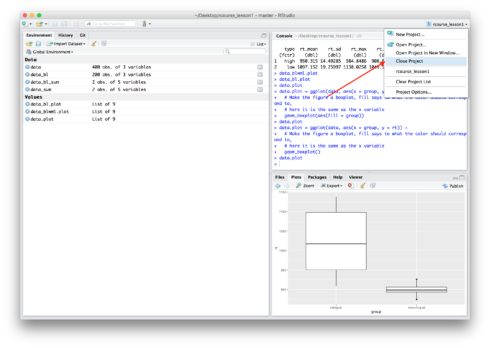
If you are done with the lesson you can also close the project. It’s important to close projects, otherwise you might start working on a new analysis in an unrelated R Project. To close your project go to the dropdown menu where your project name is written and click “Close Project”. An example screen shot is provided below.
Conclusion and Next Steps
We got through a lot today, congrats! You can now do a lot of basic functions in R in a very sophisticated way, and you can summarize you work in a nice document to share with the world. If you want to keep going with this Project look at my full script linked to at the top of the lesson. You’ll see I made a second figure with just the bilinguals and a third figure with a different way to visualize the original data. I also computed some descriptive statistics using dplyr‘s group_by() and summarise() calls. We’ll be using more dplyr code throughout the course, but if you’d like a jump start I highly recommend Hadley Wickham’s tutorial at useR 2014. Happy coding!
