Logistic regression is a machine learning algorithm which is primarily used for binary classification. In linear regression we used equation $$ p(X) = β_{0} + β_{1}X $$
The problem is that these predictions are not sensible for classification since of course, the true probability must fall between 0 and 1. To avoid this problem, we must model p(X) using a function that gives outputs between 0 and 1 for all values of X. Logistic regression is named after the function used at its core, the logistic function:
$$ p(X)=\frac{e^{β_{0} + β_{1}X }}{1+e^{β_{0} + β_{1}X }} $$
We will be working with the Titanic Data Set from Kaggle. We’ll be trying to predict a classification- survival or deceased.
Let’s begin by implementing Logistic Regression in Python for classification. We’ll use a “semi-cleaned” version of the titanic data set, if you use the data set hosted directly on Kaggle, you may need to do some additional cleaning.
Import Libraries
Let’s import some libraries to get started!
Pandas and Numpy for easier analysis.
import pandas as pd
import numpy as np
Seaborn and Matplotlib for data visualization.
import matplotlib.pyplot as plt
import seaborn as sns
%matplotlib inline
The Data
Let’s start by reading in the titanic_train.csv file into a pandas dataframe.
train = pd.read_csv('titanic_train.csv')
train.info()

RangeIndex: 891 entries, 0 to 890
Data columns (total 12 columns):
PassengerId    891 non-null int64
Survived       891 non-null int64
Pclass         891 non-null int64
Name           891 non-null object
Sex            891 non-null object
Age            714 non-null float64
SibSp          891 non-null int64
Parch          891 non-null int64
Ticket         891 non-null object
Fare           891 non-null float64
Cabin          204 non-null object
Embarked       889 non-null object
dtypes: float64(2), int64(5), object(5)
Exploratory Data Analysis
Let’s begin some exploratory data analysis! We’ll start by checking out missing data!
Missing Data
We can use seaborn to create a simple heatmap to see where we are missing data!
sns.heatmap(train.isnull(),yticklabels=False,cbar=False,cmap='viridis')
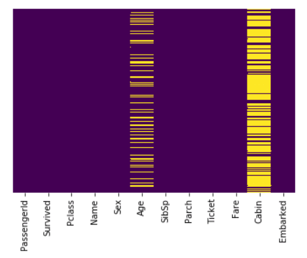
Roughly 20 percent of the Age data is missing. The proportion of Age missing is likely small enough for reasonable replacement with some form of imputation. Looking at the Cabin column, it looks like we are just missing too much of that data to do something useful with at a basic level. We’ll probably drop this later, or change it to another feature like “Cabin Known: 1 or 0”
Let’s continue on by visualizing some more of the data!
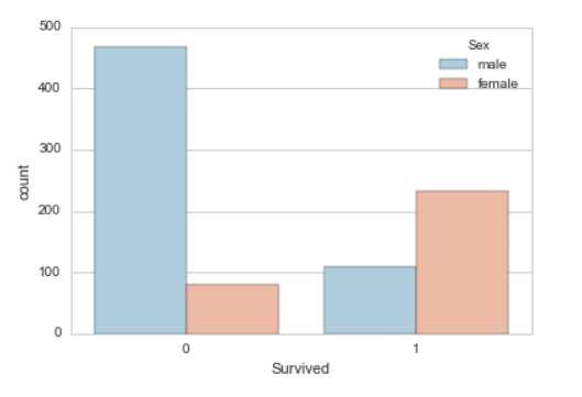
Countplot of people who survived based on their sex.
sns.countplot(x='Survived',hue='Sex',data=train,palette='RdBu_r')
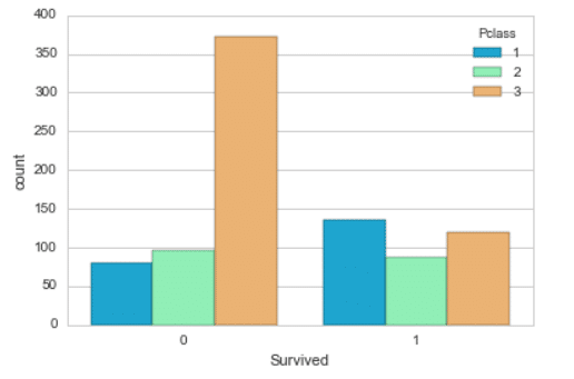
Countplot of people who survived based on their Passenger class.
sns.countplot(x='Survived',hue='Pclass',data=train,palette='rainbow')
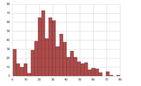
Distribution plot of dataset based on age.
train['Age'].hist(bins=30,color='darkred',alpha=0.7)
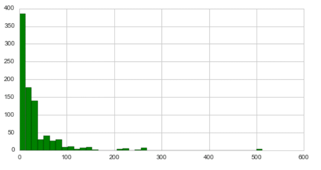
Distribution plot of different amount of fare paid by passengers.
train['Fare'].hist(color='green',bins=40,figsize=(8,4))
Data Cleaning
We want to fill in missing age data instead of just dropping the missing age data rows. One way to do this is by filling in the mean age` of all the passengers (imputation). However we can be smarter about this and check the average age by passenger class. For example:
sns.boxplot(x='Pclass',y='Age',data=train,palette='winter')
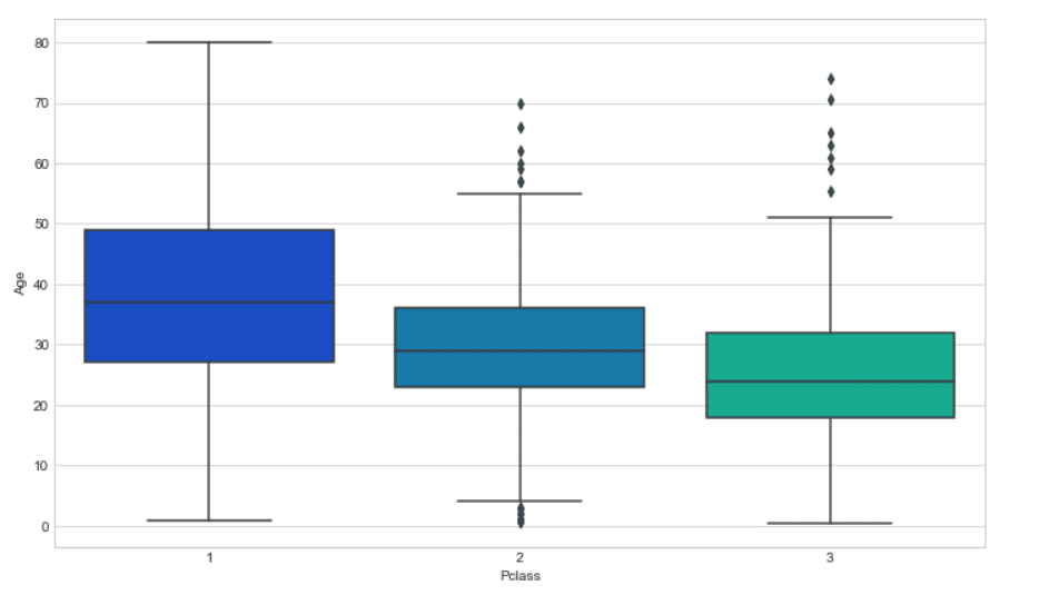
We can see the wealthier passengers in the higher classes tend to be older, which makes sense. We’ll use these average age values to impute based on Pclass for Age.
def impute_age(cols):
    Age = cols[0]
    Pclass = cols[1]

    if pd.isnull(Age):

        if Pclass == 1:
            return 37

        elif Pclass == 2:
            return 29

        else:
            return 24

    else:
        return Age

train['Age'] = train[['Age','Pclass']].apply(impute_age,axis=1)
Check that heat map again!
sns.heatmap(train.isnull(),yticklabels=False,cbar=False,cmap='viridis')
Let’s go ahead and drop the Cabin column and the row in Embarked that is NaN.
train.drop('Cabin',axis=1,inplace=True)
train.dropna(inplace=True)
Converting Categorical Features
We’ll need to convert categorical features to dummy variables using pandas! Otherwise our machine learning algorithm won’t be able to directly take in those features as inputs.
sex = pd.get_dummies(train['Sex'],drop_first=True)
embark = pd.get_dummies(train['Embarked'],drop_first=True)

train.drop(['Sex','Embarked','Name','Ticket'],axis=1,inplace=True)

train = pd.concat([train,sex,embark],axis=1)
Great! Our data is ready for our model!
Building a Logistic Regression model
Let’s start by splitting our data into a training set and test set (there is another test.csv file that you can play around with in case you want to use all this data for training).
Train Test Split
from sklearn.model_selection import train_test_split
X_train, X_test, y_train, y_test = train_test_split(train.drop('Survived',axis=1),
                                                    train['Survived'], test_size=0.30,
                                                    random_state=101)
Training and Predicting
from sklearn.linear_model import LogisticRegression
logmodel = LogisticRegression()
logmodel.fit(X_train,y_train)
predictions = logmodel.predict(X_test)
LogisticRegression(C=1.0, class_weight=None, dual=False, fit_intercept=True,
          intercept_scaling=1, max_iter=100, multi_class='ovr', n_jobs=1,
          penalty='l2', random_state=None, solver='liblinear', tol=0.0001,
          verbose=0, warm_start=False)
Let’s move on to evaluate our model!
Evaluation
We can check precision,recall,f1-score using classification report!
from sklearn.metrics import classification_reportprint(classification_report(y_test,predictions))
precision    recall  f1-score   support

          0       0.81      0.93      0.86       163
          1       0.85      0.65      0.74       104

avg / total       0.82      0.82      0.81       267
This was a brief overview of how to use a logistic regression model with python. I also demonstrated some useful methods to while doing data cleaning. The following notebook can be found here on github.
Thank You!