In my previous article i talked about Logistic Regression , a classification algorithm. In this article we will explore another classification algorithm which is K-Nearest Neighbors (KNN). We will see it’s implementation with python.
K Nearest Neighbors is a classification algorithm that operates on a very simple principle. It is best shown through example! Imagine we had some imaginary data on Dogs and Horses, with heights and weights.
Training Algorithm:
- Store all the Data
Prediction Algorithm:
- Calculate the distance from x to all points in your data
- Sort the points in your data by increasing distance from x
- Predict the majority label of the “k” closest points
Choosing a K will affect what class a new point is assigned to:
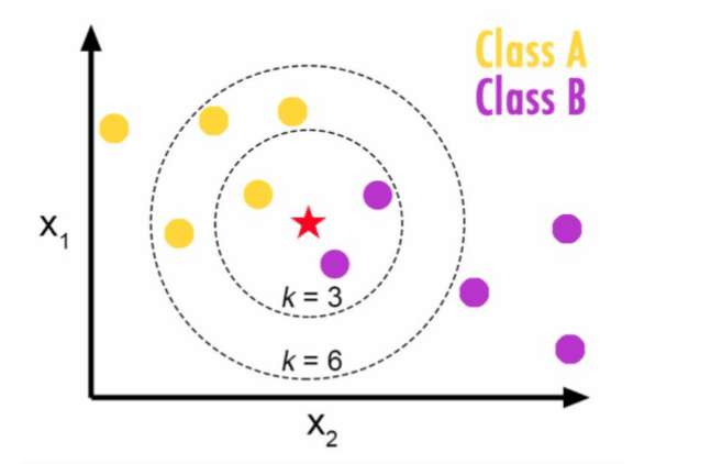
In above example if k=3 then new point will be in class B but if k=6 then it will in class A. Because majority of points in k=6 circle are from class A.
Lets return back to our imaginary data on Dogs and Horses:
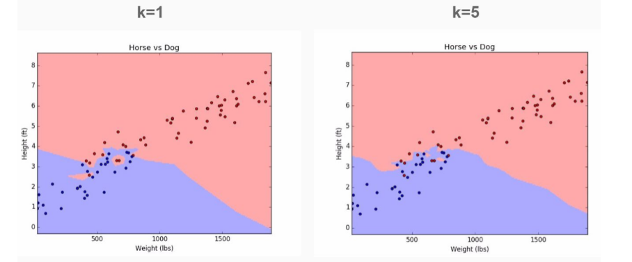
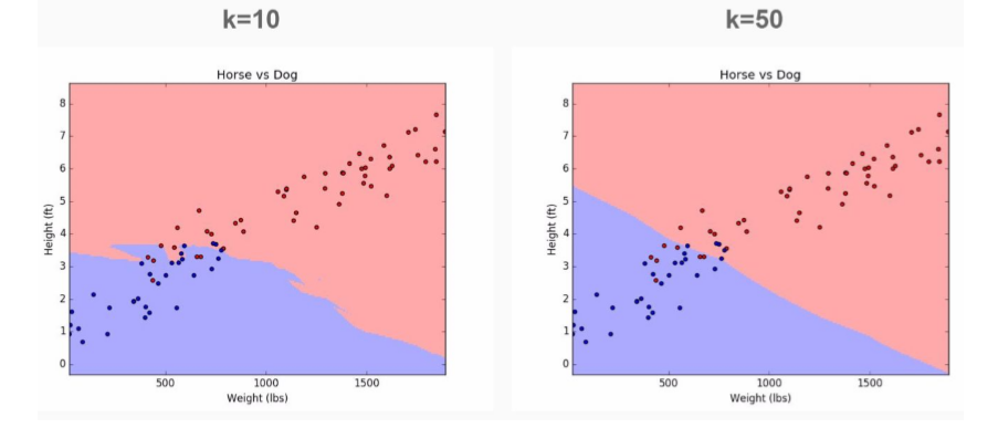
If we choose k=1 we will pick up a lot of noise in the model. But if we increase value of k, you’ll notice that we achieve smooth separation or bias. This cleaner cut-off is achieved at the cost of miss-labeling some data points.
You can read more about Bias variance tradeoff.
Pros:
- Very simple
- Training is trivial
- Works with any number of classes
- Easy to add more data
- Few parameters ○ K ○ Distance Metric
Cons:
- High Prediction Cost (worse for large data sets)
- Not good with high dimensional data
- Categorical Features don’t work well
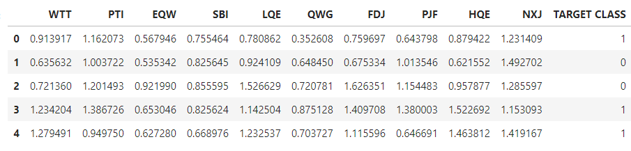
Suppose we’ve been given a classified data set from a company! They’ve hidden the feature column names but have given you the data and the target classes. We’ll try to use KNN to create a model that directly predicts a class for a new data point based off of the features.
Let’s grab it and use it!
Import Libraries
import pandas as pd
import seaborn as sns
import matplotlib.pyplot as plt
import numpy as np
%matplotlib inline
Get the Data
Set index_col=0 to use the first column as the index.
df = pd.read_csv("Classified Data",index_col=0)
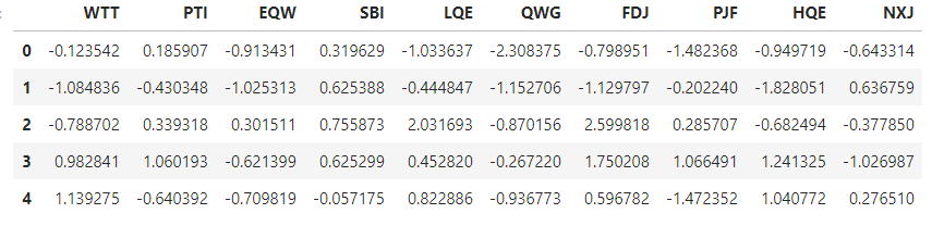
Check the head of data:
df.head()
Standardize the Variables
Because the KNN classifier predicts the class of a given test observation by identifying the observations that are nearest to it, the scale of the variables matters. Any variables that are on a large scale will have a much larger effect on the distance between the observations, and hence on the KNN classifier, than variables that are on a small scale.
from sklearn.preprocessing import StandardScaler
scaler = StandardScaler()
scaler.fit(df.drop('TARGET CLASS',axis=1))
StandardScaler(copy=True, with_mean=True, with_std=True)
scaled_features = scaler.transform(df.drop('TARGET CLASS',axis=1))
df_feat = pd.DataFrame(scaled_features,columns=df.columns[:-1])
df_feat.head()
Train Test Split
from sklearn.model_selection import train_test_split
X_train, X_test, y_train, y_test = train_test_split(scaled_features,df['TARGET CLASS'],
                                                    test_size=0.30)
Using KNN
Remember that we are trying to come up with a model to predict whether someone will TARGET CLASS or not. We’ll start with k=1.
from sklearn.neighbors import KNeighborsClassifier
knn = KNeighborsClassifier(n_neighbors=1)
knn.fit(X_train,y_train)
KNeighborsClassifier(algorithm='auto', leaf_size=30, metric='minkowski',
           metric_params=None, n_jobs=1, n_neighbors=1, p=2,
           weights='uniform')
Predictions and Evaluations
pred = knn.predict(X_test)pred = knn.predict(X_test)
Let’s evaluate our KNN model!
from sklearn.metrics import classification_report,confusion_matrix
print(confusion_matrix(y_test,pred))
[[129  12]
 [ 15 144]]
print(classification_report(y_test,pred))
  precision    recall  f1-score   support

          0       0.90      0.91      0.91       141
          1       0.92      0.91      0.91       159

avg / total       0.91      0.91      0.91       300
Choosing a K Value
Let’s go ahead and use the elbow method to pick a good K Value. We will basically check the error rate for k=1 to say k=40. For every value of k we will call KNN classifier and then choose the value of k which has the least error rate.
error_rate = []
# Might take some time
for i in range(1,40):

    knn = KNeighborsClassifier(n_neighbors=i)
    knn.fit(X_train,y_train)
    pred_i = knn.predict(X_test)
    error_rate.append(np.mean(pred_i != y_test))
Let’s plot a Line graph of the error rate.
plt.figure(figsize=(10,6))
plt.plot(range(1,40),error_rate,color='blue', linestyle='dashed', marker='o',
         markerfacecolor='red', markersize=10)
plt.title('Error Rate vs. K Value')
plt.xlabel('K')
plt.ylabel('Error Rate')
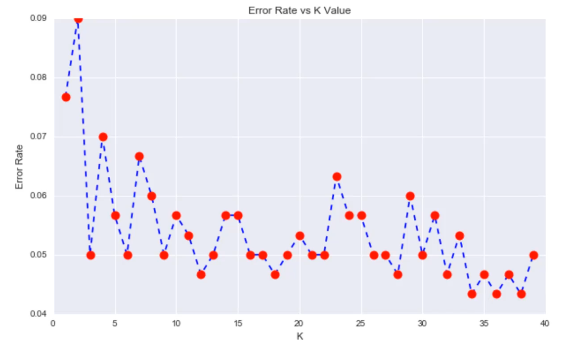
Here we can see that that after around K>23 the error rate just tends to hover around 0.06-0.05 Let’s retrain the model with that and check the classification report!
# FIRST A QUICK COMPARISON TO OUR ORIGINAL K=1
knn = KNeighborsClassifier(n_neighbors=1)
knn.fit(X_train,y_train)
pred = knn.predict(X_test)
print('WITH K=1')
print('\n')
print(confusion_matrix(y_test,pred))
print('\n')
print(classification_report(y_test,pred))
WITH K=1
[[151 8]
[ 15 126]]
precision recall f1-score support
0 0.91 0.95 0.93 159
1 0.94 0.89 0.92 141
avg / total 0.92 0.92 0.92 300
# NOW WITH K=23
knn = KNeighborsClassifier(n_neighbors=23)

knn.fit(X_train,y_train)
pred = knn.predict(X_test)

print('WITH K=23')
print('\n')
print(confusion_matrix(y_test,pred))
print('\n')
print(classification_report(y_test,pred))
WITH K=23


[[150   9]
 [ 10 131]]


             precision    recall  f1-score   support

          0       0.94      0.94      0.94       159
          1       0.94      0.93      0.93       141

avg / total       0.94      0.94      0.94       300
We were able to squeeze some more performance out of our model by tuning to a better K value. The above notebook is available here on github.
Thank you!