Linear Regression with Python

Simple linear regression lives up to its name: it is a very straightforward approach for predicting a quantitative response Y on the basis of a single predictor variable X. It assumes that there is approximately a linear relationship between X and Y. Mathematically, we can write this linear relationship as
$Y ≈ β_{0} + β_{1}X$

In this Equation, $β_{0}$ and $β_{1}$ are two unknown constants that represent the intercept and slope terms in the linear model. Together, $β_{0}$ and $β_{1}$ are known as the model coeﬃcients or parameters. While Y is the dependent variable — or the variable we are trying to predict or estimate and X is the independent variable — the variable we are using to make predictions.
Simple linear regression is a useful approach for predicting a response on the basis of a single predictor variable. However, in practice we often have more than one predictor. Instead of ﬁtting a separate simple linear regression model for each predictor, a better approach is to extend the simple linear regression model so that it can directly accommodate multiple predictors. We can do this by giving each predictor a separate slope coeﬃcient in a single model. In general, suppose that we have p distinct predictors. Then the multiple linear regression model takes the form
$Y = β_{0} + β_{1}X_{1} + β_{2}X_{2} +···+ β_{p}X_{p}$

Linear Regression with Python

Scikit Learn is awesome tool when it comes to machine learning in Python. It has many learning algorithms, for regression, classification, clustering and dimensionality reduction. In order to use Linear Regression, we need to import it:

from sklearn.linear_model import LinearRegression
Copy

We will use boston dataset.

from sklearn.datasets import load_boston
boston = load_boston()
print(boston.DESCR)
Boston House Prices dataset
===========================

Notes
------
Data Set Characteristics:  

    :Number of Instances: 506 

    :Number of Attributes: 13 numeric/categorical predictive
    
    :Median Value (attribute 14) is usually the target

    :Attribute Information (in order):
        - CRIM     per capita crime rate by town
        - ZN       proportion of residential land zoned for lots over 
                   25,000 sq.ft.
        - INDUS    proportion of non-retail business acres per town
        - CHAS     Charles River dummy variable (= 1 if tract bounds river;
                   0 otherwise)
        - NOX      nitric oxides concentration (parts per 10 million)
        - RM       average number of rooms per dwelling
        - AGE      proportion of owner-occupied units built prior to 1940
        - DIS      weighted distances to five Boston employment centres
        - RAD      index of accessibility to radial highways
        - TAX      full-value property-tax rate per $10,000
        - PTRATIO  pupil-teacher ratio by town
        - B        1000(Bk - 0.63)^2 where Bk is the proportion of blacks 
                   by town
        - LSTAT    % lower status of the population
        - MEDV     Median value of owner-occupied homes in $1000's

Copy

We should load the data as a pandas data frame and numpy for easier analysis:

import pandas as pd
import numpy as np
boston_df = boston.data
boston_df = pd.DataFrame(boston_df,columns=boston.feature_names)
Copy

We will put target column in another dataframe

target = pd.DataFrame(boston.target, columns=["MEDV"])
Copy

We should import matplotlib and seaborn for visualization.

import matplotlib.pyplot as plt
import seaborn as sns
%matplotlib inline
Copy

Check out the Data and EDA

boston_df.info()

RangeIndex: 506 entries, 0 to 505
Data columns (total 13 columns):
CRIM       506 non-null float64
ZN         506 non-null float64
INDUS      506 non-null float64
CHAS       506 non-null float64
NOX        506 non-null float64
RM         506 non-null float64
AGE        506 non-null float64
DIS        506 non-null float64
RAD        506 non-null float64
TAX        506 non-null float64
PTRATIO    506 non-null float64
B          506 non-null float64
LSTAT      506 non-null float64
dtypes: float64(13)
memory usage: 51.5 KB

Copy

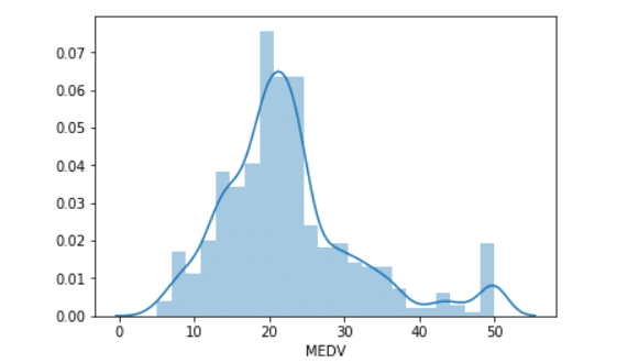
Distribution plot of median house pricing.

sns.distplot(target['MEDV'])
Copy

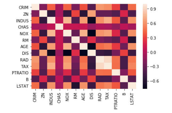
Correlation plot between all feature columns

sns.heatmap(USAhousing.corr())
Copy

Training a Linear Regression Model

Let’s now begin to train out regression model! We will need to first split up our data into an X array that contains the features to train on, and a y array with the target variable, in this case the Price column.

X and y arrays

X = boston_df[['CRIM', 'ZN', 'INDUS', 'CHAS', 'NOX', 'RM', 'AGE', 'DIS', 
               'RAD', 'TAX', 'PTRATIO', 'B', 'LSTAT']]
y = target['MEDV']
Copy

Train Test Split

Now let’s split the data into a training set and a testing set. We will train out model on the training set and then use the test set to evaluate the model.

from sklearn.model_selection import train_test_split
X_train, X_test, y_train, y_test = train_test_split(X, y, 
                                   test_size=0.4, random_state=101)
Copy

Creating and Training the Model

lm = LinearRegression()
lm.fit(X_train,y_train)
LinearRegression(copy_X=True, fit_intercept=True, n_jobs=1, normalize=False)

Copy

Model Evaluation

Let’s evaluate the model by checking out it’s coefficients and how we can interpret them.

# print the intercept
print(lm.intercept_)
41.28149654473749

Copy

coeff_df = pd.DataFrame(lm.coef_,X.columns,columns='Coefficient'])
coeff_df
Copy

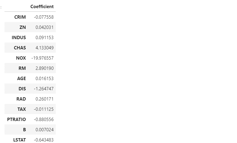
Interpreting the coefficients:
Median value of owner-occupied homes in $1000’s

Holding all other features fixed, a 1 unit increase in RM – average number of rooms per dwelling is associated with an increase of \$2890.190 .
Holding all other features fixed, a 1 unit increase in DIS – weighted distances to five Boston employment centres is associated with an decrease of \$1264.747 .
Holding all other features fixed, a 1 unit increase in PTRATIO – pupil-teacher ratio by town is associated with an decrease of \$880.556 .

Similarly all other features can be interpreted.

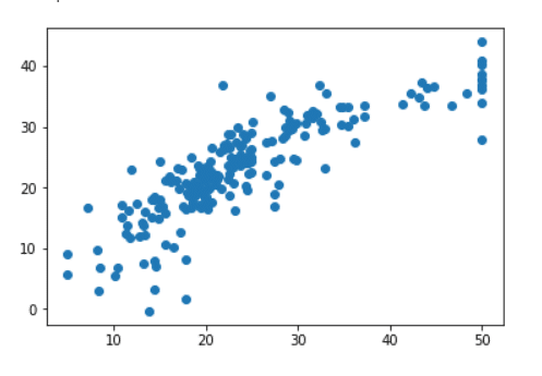
Predictions from our Model

Let’s grab predictions off our test set and see how well it did!

predictions = lm.predict(X_test)
plt.scatter(y_test,predictions)
Copy

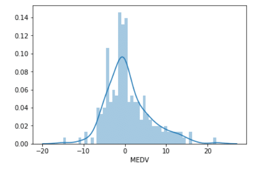
Residual Histogram

sns.distplot((y_test-predictions),bins=50);
Copy

Here are three common evaluation metrics for regression problems:
Mean Absolute Error (MAE) is the mean of the absolute value of the errors:

$\frac 1n\sum_{i=1}^n|y_i-\hat{y}_i|$

Mean Squared Error (MSE) is the mean of the squared errors:

$\frac 1n\sum_{i=1}^n(y_i-\hat{y}_i)^2$

Root Mean Squared Error (RMSE) is the square root of the mean of the squared errors:

$\sqrt{\frac 1n\sum_{i=1}^n(y_i-\hat{y}_i)^2}$
Comparing these metrics:
MAE is the easiest to understand, because it’s the average error.
MSE is more popular than MAE, because MSE “punishes” larger errors, which tends to be useful in the real world.
RMSE is even more popular than MSE, because RMSE is interpretable in the “y” units.

All of these are loss functions, because we want to minimize them.

from sklearn import metrics
print('MAE:', metrics.mean_absolute_error(y_test, predictions))
print('MSE:', metrics.mean_squared_error(y_test, predictions))
print('RMSE:', np.sqrt(metrics.mean_squared_error(y_test, predictions)))
MAE: 3.9013241932147342
MSE: 29.412643812352837
RMSE: 5.423342494472651

Copy

We’ll let this end here for now, but go ahead and explore the Boston Dataset if it is interesting to you. The above jupyter notebook is available here.

Thank you!

Data VisualisationLinear RegressionMachine Learning