In this post I will show how to build a linear regression model. As an example, for this post, I will evaluate the association between vitamin D and calcium in the blood, given that the variable of interest (i.e., calcium levels) is continuous and the linear regression analysis must be used. I will also construct multivariable-adjusted models to account for confounders.
Let's start loading the packages:
library(tidyverse)
library(RNHANES)
library(ggplot2)
Variables selected for this analysis include age, sex, plasma levels of vitamin D, and plasma levels of calcium. All variables are assessed from NHANES 2007 to 2010 wave.
d07 = nhanes_load_data("DEMO_E", "2007-2008") %>%
  select(SEQN, cycle, RIAGENDR, RIDAGEYR) %>%
  transmute(SEQN=SEQN, wave=cycle, RIAGENDR, RIDAGEYR) %>%
  left_join(nhanes_load_data("VID_E", "2007-2008"), by="SEQN") %>%
  select(SEQN, wave, RIAGENDR, RIDAGEYR, LBXVIDMS) %>%
  transmute(SEQN, wave, RIAGENDR, RIDAGEYR, vitD=LBXVIDMS) %>%
  left_join(nhanes_load_data("BIOPRO_E", "2007-2008"), by="SEQN") %>%
  select(SEQN, wave, RIAGENDR, RIDAGEYR, vitD, LBXSCA) %>%
  transmute(SEQN, wave, RIAGENDR, RIDAGEYR, vitD, Calcium = LBXSCA)

d09 = nhanes_load_data("DEMO_F", "2009-2010") %>%
  select(SEQN, cycle, RIAGENDR, RIDAGEYR) %>%
  transmute(SEQN=SEQN, wave=cycle, RIAGENDR, RIDAGEYR) %>%
  left_join(nhanes_load_data("VID_F", "2009-2010"), by="SEQN") %>%
  select(SEQN, wave, RIAGENDR, RIDAGEYR, LBXVIDMS) %>%
  transmute(SEQN, wave, RIAGENDR, RIDAGEYR, vitD=LBXVIDMS) %>%
  left_join(nhanes_load_data("BIOPRO_F", "2009-2010"), by="SEQN") %>%
  select(SEQN, wave, RIAGENDR, RIDAGEYR, vitD,  LBXSCA) %>%
  transmute(SEQN, wave, RIAGENDR, RIDAGEYR, vitD, Calcium = LBXSCA)

dat = rbind(d07, d09)

all = dat %>%
  # exclude missings
  filter(!is.na(vitD), !is.na(Calcium)) %>%
  mutate(Gender = recode_factor(RIAGENDR,
                           `1` = "Males",
                           `2` = "Females"))

head(all)
##    SEQN      wave RIAGENDR RIDAGEYR vitD Calcium  Gender
## 1 41475 2007-2008        2       62 58.8     9.5 Females
## 2 41477 2007-2008        1       71 81.8    10.0   Males
## 3 41479 2007-2008        1       52 78.4     9.0   Males
## 4 41482 2007-2008        1       64 61.9     9.1   Males
## 5 41483 2007-2008        1       66 53.3     8.9   Males
## 6 41485 2007-2008        2       30 39.1     9.3 Females
The dataset is complete. Before running the regression analysis, the linear model, I will check the assumption, that the distribution of the dependent variable (levels of calcium) is normal.
Distribution of calcium level:
ggplot(data = all) +
  geom_histogram(aes(Calcium), binwidth = 0.2)

It is a normal distribution.
Note: If the distribution is not normal, the dependant variable should be log transform by using log(Calcium).
The model
I will use the function lm() to create a linear regression model. In the first model I will not adjust for confunders, insted, I will do a univariate model.
fit1 <- lm(Calcium ~ vitD, data = all)
Now, I will plot the distribution of residuals to check for normality.
hist(residuals(fit1))
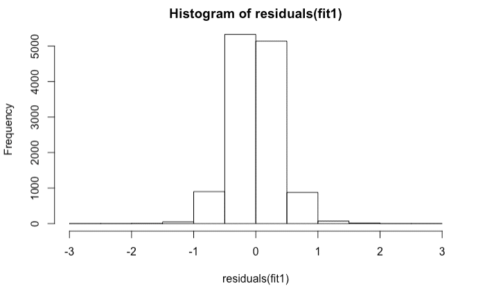
It is normally distributed.
To see the results, estimates, pvalues etc use summary function.
summary(fit1)
##
## Call:
## lm(formula = Calcium ~ vitD, data = all)
##
## Residuals:
##      Min       1Q   Median       3Q      Max
## -2.51254 -0.23398 -0.00581  0.22943  2.64876
##
## Coefficients:
##              Estimate Std. Error t value Pr(>|t|)
## (Intercept) 9.3517792  0.0087769 1065.50   <2e-16 ***
## vitD        0.0016522  0.0001315   12.56   <2e-16 ***
## ---
## Signif. codes:  0 '***' 0.001 '**' 0.01 '*' 0.05 '.' 0.1 ' ' 1
##
## Residual standard error: 0.3683 on 12389 degrees of freedom
## Multiple R-squared:  0.01258,    Adjusted R-squared:  0.0125
## F-statistic: 157.8 on 1 and 12389 DF,  p-value: < 2.2e-16
The 95% confidence interval:
confint(fit1)
##                   2.5 %      97.5 %
## (Intercept) 9.334575125 9.368983370
## vitD        0.001394404 0.001910026
Intepretation
From the results, I find that vitamin D is associated with calcium in the blood because the p-value is less than 0.05. Next, I see the direction of the association. The positive beta estimate (\(\beta\) = 0.0016) indicate that with increasing vitamin D in the blood, the levels of calcium also increases.
To visualize this association I will use the ggplot and the function geom_smooth. See below:
ggplot(all, aes(x = vitD, y = Calcium)) +
            geom_point() +
            geom_smooth(method="lm")

The plot shows an increase of the levels of Calcium with the increase of vitamin D in the blood.
Multivariable adjusted models
Often, a significant association could be explained by confounders. According to Wikipedia, a confounder is a variable that influences both the dependent variable and independent variable, causing a spurious association. Therefore, it is important to adjust for major confounders such as age and gender. The levels of vitamin D in the blood are dependent to age because older adults have lower vitamin D in blood compared to young adults.
To conduct a multivariable-adjusted model I add other variables to the model, in this example, I will add age and gender.
fit2 <- lm(Calcium ~ vitD + Gender + RIDAGEYR, data = all)
summary(fit2)
##
## Call:
## lm(formula = Calcium ~ vitD + Gender + RIDAGEYR, data = all)
##
## Residuals:
##      Min       1Q   Median       3Q      Max
## -2.50114 -0.22824 -0.00857  0.22354  2.69352
##
## Coefficients:
##                 Estimate Std. Error t value Pr(>|t|)
## (Intercept)    9.4686333  0.0109933 861.307   <2e-16 ***
## vitD           0.0019034  0.0001310  14.526   <2e-16 ***
## GenderFemales -0.0653111  0.0065383  -9.989   <2e-16 ***
## RIDAGEYR      -0.0022455  0.0001581 -14.204   <2e-16 ***
## ---
## Signif. codes:  0 '***' 0.001 '**' 0.01 '*' 0.05 '.' 0.1 ' ' 1
##
## Residual standard error: 0.3639 on 12387 degrees of freedom
## Multiple R-squared:  0.03619,    Adjusted R-squared:  0.03596
## F-statistic: 155.1 on 3 and 12387 DF,  p-value: < 2.2e-16
The association between vitamin D and calcium remained significant after adjustment, suggesting that the association is independent (e.g., not explained) by age and gender.
Stratifing analysis
To evaluate the association separately in men and women is necessary to conduct a stratified analysis. For this, I need to separate men and women into two different datasets and run linear regression for each group.
allfem = all %>%
  filter(Gender == "Females")
allmal = all %>%
  filter(Gender == "Males")
Linear regression in women and men
fitfem <- lm(Calcium ~ vitD + RIDAGEYR, data = allfem)
summary(fitfem)
##
## Call:
## lm(formula = Calcium ~ vitD + RIDAGEYR, data = allfem)
##
## Residuals:
##      Min       1Q   Median       3Q      Max
## -2.03557 -0.24115 -0.01084  0.22396  2.61555
##
## Coefficients:
##              Estimate Std. Error t value Pr(>|t|)
## (Intercept) 9.2764092  0.0145412 637.940   <2e-16 ***
## vitD        0.0019577  0.0001729  11.321   <2e-16 ***
## RIDAGEYR    0.0005348  0.0002307   2.318   0.0205 *
## ---
## Signif. codes:  0 '***' 0.001 '**' 0.01 '*' 0.05 '.' 0.1 ' ' 1
##
## Residual standard error: 0.3727 on 6254 degrees of freedom
## Multiple R-squared:  0.02247,    Adjusted R-squared:  0.02216
## F-statistic: 71.89 on 2 and 6254 DF,  p-value: < 2.2e-16
fitmal <- lm(Calcium ~ vitD + RIDAGEYR, data = allmal)
summary(fitmal)
##
## Call:
## lm(formula = Calcium ~ vitD + RIDAGEYR, data = allmal)
##
## Residuals:
##      Min       1Q   Median       3Q      Max
## -2.42787 -0.21555 -0.00506  0.21384  2.70896
##
## Coefficients:
##               Estimate Std. Error t value Pr(>|t|)
## (Intercept)  9.6027158  0.0150801  636.78   <2e-16 ***
## vitD         0.0016591  0.0001973    8.41   <2e-16 ***
## RIDAGEYR    -0.0049452  0.0002105  -23.49   <2e-16 ***
## ---
## Signif. codes:  0 '***' 0.001 '**' 0.01 '*' 0.05 '.' 0.1 ' ' 1
##
## Residual standard error: 0.3451 on 6131 degrees of freedom
## Multiple R-squared:  0.08713,    Adjusted R-squared:  0.08684
## F-statistic: 292.6 on 2 and 6131 DF,  p-value: < 2.2e-16
The interpretation of results should be as above.
Thats all.