Using kNN Classifier to Predict Whether the Price of Stock Will Increase

In this article, I will show you how to use the k-Nearest Neighbors algorithm (kNN for short) to predict whether price of Apple stock will increase or decrease. I obtained the data from Yahoo Finance. You can download the dataset here.

What is the k-Nearest Neighbors algorithm?

The kNN algorithm is a non-parametric algorithm that can be used for either classification or regression. Non-parametric means that it makes no assumption about the underlying data or its distribution. It is one of the simplest Machine Learning algorithms, and has applications in a variety of fields, ranging from the healthcare industry, to the finance industry. Since we will use it for classification here, I will explain how it works as a classifier.

For each data point, the algorithm finds the k closest observations, and then classifies the data point to the majority. Usually, the k closest observations are defined as the ones with the smallest Euclidean distance to the data point under consideration. For example, if k = 3, and the three nearest observations to a specific data point belong to the classes A, B, and A respectively, the algorithm will classify the data point into class A. If k is even, there might be ties. To avoid this, usually weights are given to the observations, so that nearer observations are more influential in determining which class the data point belongs to. An example of this system is giving a weight of 1/d to each of the observations, where d is distance to the data point. If there is still a tie, then the class is chosen randomly.

Building the model

The knn function is available in the class library. Apart from that, we will also need the dplyr and lubridate library. We also need to set the seed to ensure our results are reproducible, because in case of ties, the results will be randomized (as explained above). Let’s load up the data and take a look!

library(class)
library(dplyr)
library(lubridate)
set.seed(100)

stocks <- read.csv('stocks.csv')

        Date  Apple Google  MSFT Increase
1 2010-01-04 214.01 626.75 30.95     TRUE
2 2010-01-05 214.38 623.99 30.96     TRUE
3 2010-01-06 210.97 608.26 30.77    FALSE
4 2010-01-07 210.58 594.10 30.45    FALSE
5 2010-01-08 211.98 602.02 30.66     TRUE
6 2010-01-11 210.11 601.11 30.27    FALSE

Here, the 3 columns represent the closing price of the stock of their respective companies on the given date. The Increase column represents whether the price of Apple rose or fell as compared to the previous day.

If you look at the help file for knn using ?knn, you will see that we have to provide the testing set, training set, and the classification vector all at the same time. For most other prediction algorithms, we build the prediction model on the training set in the first step, and then use the model to test our predictions on the test set in the second step. However, the kNN function does both in a single step. Let us put all data before the year 2014 into the training set, and the rest into the test set.

stocks$Date <- ymd(stocks$Date)
stocksTrain <- year(stocks$Date) < 2014

Now, we need to build the training set. It will consist of the prices of stocks of Apple, Google, and Microsoft on the previous day. For this, we can use the lag function in dplyr.

predictors <- cbind(lag(stocks$Apple, default = 210.73), lag(stocks$Google, default = 619.98), lag(stocks$MSFT, default = 30.48))

Since for the very first value (corresponding to January 4, 2010), the lag function has nothing to compare it to, it will default to NA. To avoid this, I set the default values for each stock to be its value on the previous business day (December 31, 2009).

Now, let’s build the prediction model.

prediction <- knn(predictors[stocksTrain, ], predictors[!stocksTrain, ], stocks$Increase[stocksTrain], k = 1)

We can see it’s accuracy using table.

table(prediction, stocks$Increase[!stocksTrain])

prediction FALSE TRUE
     FALSE    29   32
     TRUE    192  202

and we can measure it’s accuracy as follows:

mean(prediction == stocks$Increase[!stocksTrain])

[1] 0.5076923

This is only marginally better than random guessing (50%). Let’s see if we can get a better accuracy by changing the value of k. We can use a for loop to see how the algorithm performs for different values of k.

accuracy <- rep(0, 10)
k <- 1:10
for(x in k){
  prediction <- knn(predictors[stocksTrain, ], predictors[!stocksTrain, ],
                    stocks$Increase[stocksTrain], k = x)
  accuracy[x] <- mean(prediction == stocks$Increase[!stocksTrain])
}

plot(k, accuracy, type = 'b')

This gives the following graph:

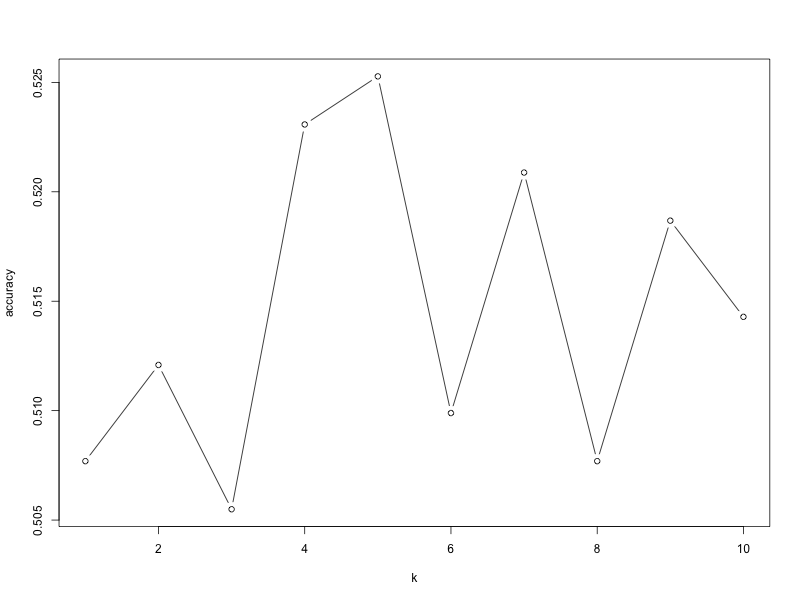
As we can see, the model has the highest accuracy of ~52.5% when k = 5. While this may not seem any good, it is often extremely hard to predict the price of stocks. Even the 2.5% improvement over random guessing can make a difference given the amount of money at stake. After all, if it was that easy to predict the prices, wouldn’t we all be trading in stocks for the easy money instead of learning these algorithms?

That brings us to the end of this post. I hope you enjoyed it. Feel free to leave a comment or reach out to me on Twitter if you have questions!

Note: If you are interested in learning more, I highly recommend reading Introduction to Statistical Learning (a pdf copy of the book is available for free on the website).

AlgorithmdplyrK-Nearest NeighborsMachine LearningPrediction