According to Wikipedia, propensity score matching (PSM) is a “statistical matching technique that attempts to estimate the effect of a treatment, policy, or other intervention by accounting for the covariates that predict receiving the treatment”. In a broader sense, propensity score analysis assumes that an unbiased comparison between samples can only be made when the subjects of both samples have similar characteristics. Thus, PSM can not only be used as “an alternative method to estimate the effect of receiving treatment when random assignment of treatments to subjects is not feasible” (Thavaneswaran 2008). It can also be used for the comparison of samples in epidemiological studies. Let’s give an example:
Health-related quality of life (HRQOL) is considered an important outcome in cancer therapy. One of the most frequently used instruments to measure HRQOL in cancer patients is the core quality-of-life questionnaire of the European Organisation for Research and Treatment of Cancer. The EORTC QLQ-C30 is a 30-item instrument comprised of five functioning scales, nine symptom scales and one scale measuring Global quality of life. All scales have a score range between 0 and 100. While high scores of the symptom scales indicate a high burden of symptoms, high scores of the functioning scales and on the GQoL scale indicate better functioning resp. quality of life.
However, without having any reference point, it is difficult if not impossible to interpret the scores. Fortunately, the EORTC QLQ-C30 questionnaire was used in several general population surveys. Therefore, patient scores may be compared against scores of the general population. This makes it far easier to decide whether the burden of symptoms or functional impairments can be attributed to cancer (treatment) or not. PSM can be used to make both patient and population samples comparable by matching for relevant demographic characteristics like age and sex.
In this blog post, I show how to do PSM using R. A more comprehensive PSM guide can be found under: “A Step-by-Step Guide to Propensity Score Matching in R“.
Creating two random dataframes
Since we don’t want to use real-world data in this blog post, we need to emulate the data. This can be easily done using the Wakefield package.
In a first step, we create a dataframe named df.patients. We want the dataframe to contain specifications of age and sex for 250 patients. The patients’ age shall be between 30 and 78 years. Furthermore, 70% of patients shall be male.
set.seed(1234)
df.patients <- r_data_frame(n = 250,
                            age(x = 30:78,
                                name = 'Age'),
                            sex(x = c("Male", "Female"),
                                prob = c(0.70, 0.30),
                                name = "Sex"))
df.patients$Sample <- as.factor('Patients')
The summary-function returns some basic information about the dataframe created. As we can see, the mean age of the patient sample is 53.7 and roughly 70% of the patients are male (69.2%).
summary(df.patients)
##       Age            Sex           Sample
##  Min.   :30.00   Male  :173   Patients:250
##  1st Qu.:42.00   Female: 77
##  Median :54.00
##  Mean   :53.71
##  3rd Qu.:66.00
##  Max.   :78.00
In a second step, we create another dataframe named df.population. We want this dataframe to comprise the same variables as df.patients with different specifications. With 18 to 80, the age-range of the population shall be wider than in the patient sample and the proportion of female and male patients shall be the same.
set.seed(1234)
df.population <- r_data_frame(n = 1000,
                              age(x = 18:80,
                                  name = 'Age'),
                              sex(x = c("Male", "Female"),
                                  prob = c(0.50, 0.50),
                                  name = "Sex"))
df.population$Sample <- as.factor('Population')
The following table shows the sample’s mean age (49.5 years) and the proportion of men (48.5%) and women (51.5%).
summary(df.population)
##       Age            Sex             Sample
##  Min.   :18.00   Male  :485   Population:1000
##  1st Qu.:34.00   Female:515
##  Median :50.00
##  Mean   :49.46
##  3rd Qu.:65.00
##  Max.   :80.00
Merging the dataframes
Before we match the samples, we need to merge both dataframes. Based on the variable Sample, we create a new variable named Group (type logic) and a further variable (Distress) containing information about the individuals’ level of distress. The Distress variable is created using the age-function of the Wakefield package. As we can see, women will have higher levels of distress.
mydata <- rbind(df.patients, df.population)
mydata$Group <- as.logical(mydata$Sample == 'Patients')
mydata$Distress <- ifelse(mydata$Sex == 'Male', age(nrow(mydata), x = 0:42, name = 'Distress'),
                                                age(nrow(mydata), x = 15:42, name = 'Distress'))
When we compare the distribution of age and sex in both samples, we discover significant differences:
pacman::p_load(tableone)
table1 <- CreateTableOne(vars = c('Age', 'Sex', 'Distress'),
                         data = mydata,
                         factorVars = 'Sex',
                         strata = 'Sample')
table1 <- print(table1,
                printToggle = FALSE,
                noSpaces = TRUE)
kable(table1[,1:3],
      align = 'c',
      caption = 'Table 1: Comparison of unmatched samples')
Table 1: Comparison of unmatched samples
| Patients | Population | p | |
|---|---|---|---|
| n | 250 | 1000 | |
| Age (mean (sd)) | 53.71 (13.88) | 49.46 (18.33) | 0.001 |
| Sex = Female (%) | 77 (30.8) | 515 (51.5) | <0.001 |
| Distress (mean (sd)) | 22.86 (11.38) | 25.13 (11.11) | 0.004 |
Furthermore, the level of distress seems to be significantly higher in the population sample.
Matching the samples
Now, that we have completed preparation and inspection of data, we are going to match the two samples using the matchit-function of the MatchIt package. The method command method="nearest" specifies that the nearest neighbors method will be used. Other matching methods are exact matching, subclassification, optimal matching, genetic matching, and full matching (method = c("exact", "subclass", "optimal", ""genetic", "full")). The ratio command ratio = 1 indicates a one-to-one matching approach. With regard to our example, for each case in the patient sample exactly one case in the population sample will be matched. Please also note that the Group variable needs to be logic (TRUE vs. FALSE).
set.seed(1234)
match.it <- matchit(Group ~ Age + Sex, data = mydata, method="nearest", ratio=1)
a <- summary(match.it)
For further data presentation, we save the output of the summary-function into a variable named a.
After matching the samples, the size of the population sample was reduced to the size of the patient sample (n=250; see table 2).
kable(a$nn, digits = 2, align = 'c',
      caption = 'Table 2: Sample sizes')
Table 2: Sample sizes
| Control | Treated | |
|---|---|---|
| All | 1000 | 250 |
| Matched | 250 | 250 |
| Unmatched | 750 | 0 |
| Discarded | 0 | 0 |
The following output shows, that the distributions of the variables Age and Sex are nearly identical after matching.
kable(a$sum.matched[c(1,2,4)], digits = 2, align = 'c',
      caption = 'Table 3: Summary of balance for matched data')
Table 3: Summary of balance for matched data
| Means Treated | Means Control | Mean Diff | |
|---|---|---|---|
| distance | 0.23 | 0.23 | 0.00 |
| Age | 53.71 | 53.65 | 0.06 |
| SexMale | 0.69 | 0.69 | 0.00 |
| SexFemale | 0.31 | 0.31 | 0.00 |
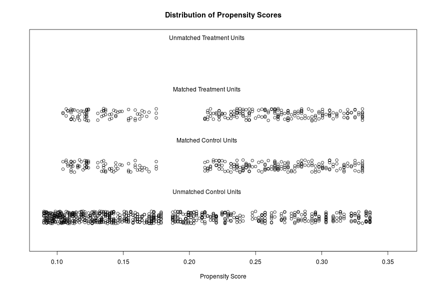
The distributions of propensity scores can be visualized using the plot-function which is part of the MatchIt package .
plot(match.it, type = 'jitter', interactive = FALSE)
Here is the plot:
Saving the matched samples
Finally, the matched samples will be saved into a new dataframe named df.match.
df.match <- match.data(match.it)[1:ncol(mydata)]
rm(df.patients, df.population)
Eventually, we can check whether the differences in the level of distress between both samples are still significant.
pacman::p_load(tableone)
table4 <- CreateTableOne(vars = c('Age', 'Sex', 'Distress'),
                         data = df.match,
                         factorVars = 'Sex',
                         strata = 'Sample')
table4 <- print(table4,
                printToggle = FALSE,
                noSpaces = TRUE)
kable(table4[,1:3],
      align = 'c',
      caption = 'Table 4: Comparison of matched samples')
| Patients | Population | p | |
|---|---|---|---|
| n | 250 | 250 | |
| Age (mean (sd)) | 53.71 (13.88) | 53.65 (13.86) | 0.961 |
| Sex = Female (%) | 77 (30.8) | 77 (30.8) | 1.000 |
| Distress (mean (sd)) | 22.86 (11.38) | 24.13 (11.88) | 0.222 |
With a p-value of 0.222, Student’s t-test does not indicate significant differences anymore. Thus, PSM helped to avoid an alpha mistake.
PS 1: The packages used in this blog post can be loaded/installed using the following code:
pacman::p_load(knitr, wakefield, MatchIt, tableone, captioner)
PS 2: Thanks very much to my colleague Katharina Kuba for telling me about the MatchIt package.