After scraping reviews from Goodreads in the first installment of this series, we are now ready to do some exploratory data analysis to get a better sense of the data we have. This will also allow us to create features that we will use in future analyses.
Setup and data preparation
We start by loading the libraries and the data from part 1, that I have consolidated in one file.
library(data.table)
library(dplyr)
library(ggplot2)
library(stringr)
library(tm)
library(magrittr)
library(textcat)
library(tidytext)
library(RTextTools)

data <- read.csv("GoodReadsData.csv", stringsAsFactors = FALSE)
data <- data.table(data)
After a quick inspection of the data, we realize that some reviews are not in English. We get rid of them.
data$language <- as.factor(textcat(data$review))
data <- data[language == "english"]
The language detection algorithm is not great and reclassifies some reviews in weird languages (6 breton? 9 rumantsch?? 103 middle frisian???), but that's good enough for what we want to do.
Then we exclude all ratings that do not correspond to a 1 to 5 star rating (such as “currently reading it”, or an empty rating) and all reviews that are too short.
data <- data[rating %in% c('did not like it',
                           'it was ok',
                           'liked it',
                           'really liked it',
                           'it was amazing')]
data <- data[length(data$review) >= 5]
Finally, we recode the ratings in numerical format, remove the language and reviewer columns that we won’t be using anymore, and add a review_id column (to be able to identify to which review a word belongs).
data$rating[data$rating == 'did not like it'] <- 1
data$rating[data$rating == 'it was ok'      ] <- 2
data$rating[data$rating == 'liked it'       ] <- 3
data$rating[data$rating == 'really liked it'] <- 4
data$rating[data$rating == 'it was amazing' ] <- 5
data$rating <- as.integer(data$rating)

data$language <- NULL
data$reviewer <- NULL
data$review.id <- 1:nrow(data)
With that, we are now ready to start exploratory data analysis!
Exploratory data analysis
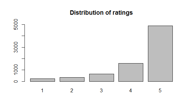
Let’s start by looking at the distribution of ratings. As we can see, the ratings are rather unbalanced, something to keep in mind in future analyses.
barplot(table(as.factor(data$rating)),
        ylim = c(0,5000),
        main = "Distribution of ratings")
The plot:
Let’s take a look at the distribution of the length of reviews.
data$review.length = nchar(data$review)
hist(data$review.length,
     ylim = c(0,5000),
     main = "Distribution of review length" )
The plot:
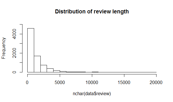
Now that’s a long tail! A quick calculation let us know that there are only 45 reviews that are more than 8000 character long. Let’s get rid of them, to avoid skewing our analyses (e.g. if one of these reviews uses a lot a word, it could bias the weight for that word).
n <- nrow(data[data$review.length >= 8000])
data <- data[data$review.length <= 8000]
hist(data$review_length,
     ylim = c(0,3000),
     main = "Distribution of review length" )
The plot:

This looks better. Finally, let’s take a look at the distribution of review length by rating.
with(data, boxplot(review.length~rating,
                   main = "Distribution of review length by rating"))
The plot:
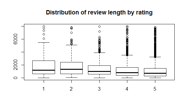
Visually, more positive reviews appear to be slightly shorter than more negative reviews, but there’s no definite trend. Let’s turn to sentiment analysis, by replicating mutatis mutandis the analyses of David Robinson on Yelp’s reviews using the tidytext package.
Sentiment analysis
In this section, we are going to use the “positive” or “negative” aspect of words (from the sentiments dataset within the tidytext package) to see if it correlates with the ratings. In order to do that, we need to start by establishing lexicons of words with a positive/negative score.
# Loading the first sentiment score lexicon
AFINN <- sentiments %>%
  filter(lexicon == "AFINN") %>%
  select(word, afinn_score = score)
head(AFINN)

# Loading the second sentiment score lexicon
Bing <- sentiments %>%
  filter(lexicon == "bing") %>%
  select(word, bing_sentiment = sentiment)
head(Bing)
We then “tidy up” our dataset by making it “tall” (one word per row) and add the sentiment scores for each word
# "tidying" up the data (1 word per row) and adding the sentiment scores for each word
review_words <- data %>%
  unnest_tokens(word, review) %>%
  select(-c(book, review_length)) %>%
  left_join(AFINN, by = "word") %>%
  left_join(Bing, by = "word")
Our data now looks like this:
| rating | review_id | word | afinn_score | bing_score |
|---|---|---|---|---|
| 5 | 1 | love | 3 | positive |
| 5 | 3381 | if | NA | NA |
| 1 | 8090 | hell | -4 | negative |
We can assign a positivity/negativity “score” to each review by calculating the average score of all the words the review (using the AFINN lexicon; using the Bing lexicon would yield a similar result).
# Grouping by mean for observation
review_mean_sentiment <- review_words %>%
  group_by(review_id, rating) %>%
  summarize(mean_sentiment = mean(afinn_score, na.rm = TRUE))
The outcome looks like this:
| review_id | rating | mean_sentiment |
|---|---|---|
| 1 | 5 | 0.9444 |
| 2 | 3 | -0.093 |
| 3 | 5 | -1.17 |
So, how does the average sentiment score vary by rating?
theme_set(theme_bw())
ggplot(review.mean.sentiment, aes(rating, mean.sentiment, group = rating)) +
  geom_boxplot() +
  ylab("Average sentiment score")
The plot:

We’re onto something! Visually at least, we can see a difference across ratings, with the sentiment score for 1-star reviews being squarely negative and the sentiment score for 5-star reviews being squarely positive. Let’s create a new dataset to integrate this feature for future use (note that some reviews are too short or use no word recorded in our lexicons, so they don’t have a score).
review.mean.sentiment <- review.mean.sentiment %>%
  select(-rating) %>% # We remove the rating here to avoid duplicating it
  data.table()
clean.data <- data %>%
  left_join(review.mean.sentiment, by = "review.id")
The difference between ratings is even clearer if we take the median score instead of the mean:
review.median.sentiment <- review.words %>%
  group_by(review.id, rating) %>%
  summarize(median.sentiment = median(afinn.score, na.rm = TRUE))
theme_set(theme_bw())
ggplot(review.median.sentiment, aes(rating, median.sentiment, group = rating)) +
  geom_boxplot() +
  ylab("Median sentiment score")
The plot:
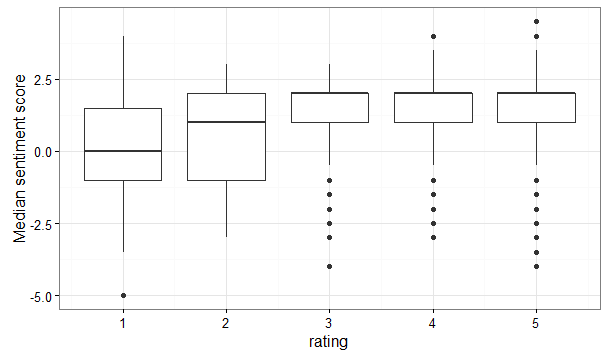
Again, let’s transfer this feature to our new dataset.
review.median.sentiment <- review.median.sentiment %>%
  select(-rating) %>%
  data.table()
clean.data <- clean.data %>%
  left_join(review.median.sentiment, by = "review.id")
Last but not least, we are going to count the number of negative and positive words in each review, according to the two lexicons, for use in the machine learning algorithm.
# Counting the number of negative words per review according to AFINN lexicon
review.count.afinn.negative <- review.words %>%
  filter(afinn.score < 0) %>%
  group_by(review.id, rating) %>%
  summarize(count.afinn.negative = n())
# Transferring the results to our dataset
review.count.afinn.negative <- review.count.afinn.negative %>%
  select(-rating) %>%
  data.table()
clean.data <- clean.data %>%
  left_join(review.count.afinn.negative, by = "review.id")

# Counting the number of positive words per review according to AFINN lexicon
review.count.afinn.positive <- review.words %>%
  filter(afinn.score > 0) %>%
  group_by(review.id, rating) %>%
  summarize(count.afinn.positive = n())
# Transferring the results to our dataset
review.count.afinn.positive <- review.count.afinn.positive %>%
  select(-rating) %>%
  data.table()
clean.data <- clean.data %>%
  left_join(review.count.afinn.positive, by = "review.id")

# Counting the number of negative words per review according to Bing lexicon
review.count.bing.negative <- review.words %>%
  filter(bing.sentiment == "negative") %>%
  group_by(review.id, rating) %>%
  summarize(count.bing.negative = n())
# Transferring the results to our dataset
review.count.bing.negative <- review.count.bing.negative %>%
  select(-rating) %>%
  data.table()
clean.data <- clean.data %>%
  left_join(review.count.bing.negative, by = "review.id")

# Counting the number of positive words per review according to Bing lexicon
review.count.bing.positive <- review.words %>%
  filter(bing.sentiment == "positive") %>%
  group_by(review.id, rating) %>%
  summarize(count.bing.positive = n())
# Transferring the results to our dataset
review.count.bing.positive <- review.count.bing.positive %>%
  select(-rating) %>%
  data.table()
clean.data <- clean.data %>%
  left_join(review.count.bing.positive, by = "review.id")
Finally, we save our data to a file for future use.
write.csv(clean.data, "GoodReadsCleanData.csv", row.names = FALSE)
Just for exploratory purposes, we are now going to slice our data the other way around, aggregating not by review but by word. First, for each word, we are going to count in how many reviews it appears and how many times it appears overall, as well as calculate the average rating of the reviews in which it appears. Finally, we filter our data to keep only the words that appears in at least 3 reviews, to avoid words that would be peculiar to a specific reviewer.
word.mean.summaries <- review.words %>%
  count(review.id, rating, word) %>%
  group_by(word) %>%
  summarize(reviews = n(),
            uses = sum(n),
            average.rating = mean(rating)) %>%
  filter(reviews >= 3) %>%
  arrange(average.rating)
The outcome looks like this:
| word | reviews | uses | average_rating |
|---|---|---|---|
| mystified | 3 | 3 | 1.6667 |
| operator | 3 | 3 | 1.6667 |
| unlikeable | 9 | 12 | 1.6667 |
And finally, we can compare the average rating in the previous table with the AFINN score for the word:
word.mean.afinn <- word.mean.summaries %>%
  inner_join(AFINN)

ggplot(word.mean.afinn, aes(afinn.score, average.rating, group = afinn.score)) +
  geom_boxplot() +
  xlab("AFINN score of word") +
  ylab("Mean rating of reviews with this word")
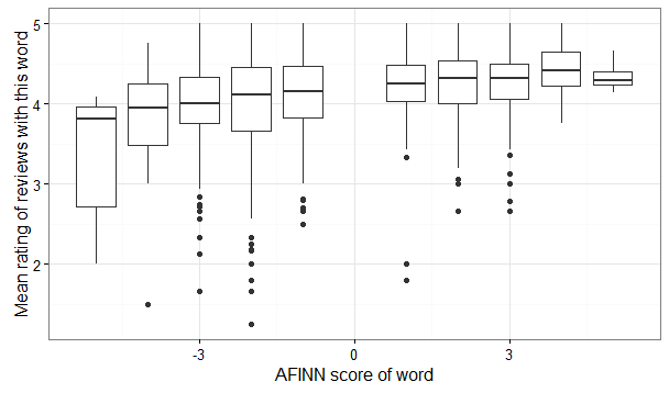
Once again, we can see that there is some correlation between the ratings and the AFINN scores, this time at the word level. The question is then: can we predict at least somewhat accurately the rating of a review based on the words of the review? That will be the topic of the last installment in this series.
As for the first installment, the complete R code is available on my github.
Hey Jasmine! The two lexicons I used come from the tidytext package. You can read more about them here: http://juliasilge.com/blog/Life-Changing-Magic/
Can you please explain what is first and second sentiment score lexicon?
Excellent analysis! Can’t wait for the next installment in this series.