In my previous post, I introduced the concept of smoothing using Fourier basis functions and I applied them onto temperature data. It is important to note the that a similar kind of analysis can be replicated using B-splines (see this page). In this post, I extend the concept to an another type of basis functions: Gaussian Radial basis functions. Radial basis functions are part of a class of single hidden layer feedforward networks which can be expressed as a linear combination of radially symmetric nonlinear basis functions. Each basis function forms a localized receptive field in the input space. The most commonly used function is the Gaussian Basis
Modeling Gaussian Basis functions
Algebraically, Gaussian basis functions are defined as follows:
$$ \phi_k(t;\mu_k ,\sigma^2_k) = \exp \left(-\dfrac{||t-\mu_k||^2}{2\sigma^2_k}\right),\textbf{ } k=1,\dots,K $$ where \(\mu_k\) is a parameter determining the center of the basis function, \(\sigma^2_k\) is a parameter that determines the width and \(||.||\) is the Euclidian norm. The basis functions overlap with each other to capture the information about \(t\), and the width parameter play an essential role to capture the structure in the data over the region of input data. The parameters featuring in each basis function are often determined heuristically based on the structure of the observed data.
K-means Clustering
Using K-means Clustering, the observational space \(\mathcal{T}\) into K clusters \(\{C_1,C_2,\dots,C_K\}\) that correspond to the number of basis functions. They are determined by:
$$\hat{\mu}_k = \frac{1}{N_k}\sum_{t_j \in C_k} t_j, \text{ and } \hat{\sigma}^2_k = \dfrac{1}{N_k}\sum_{t_j \in C_k} ||t_j – \hat{\mu}_k||^2$$ where \(N_k\) is the number of observations which belongs to the \(k^{th}\) cluster. However, this method does not produce unique parameters for a unique set of observations, due to the stochastic nature of the starting value in the clustering algorithm. Because of that feature, the K-means clustering underperforms when capturing all the information from the data. This is noticeable when the set of Functional Data are observed at equidistant points. In order to control the amount of overlapping as a mean to overcome the lack of overlapping among basis functions, we may introduce a hyper-parameter. Hence, \(\phi_k(t)\)’s are written:
$$\phi_k(t;\mu_k ,\sigma^2_k) = \exp \left(-\dfrac{||t-\mu_k||^2}{2\nu \sigma^2_k}\right),\textbf{ } k=1,\dots,K$$
In R, these basis functions are generated as below:
data(motorcycledata, package = "adlift")
mtt = motorcycledata$time # the timestamps
n = 8 # the number of basis functions over T
nyu = 5 # hyperparameter

k = kmeans(mtt, centers = n,algorithm = "Hartigan-Wong")
myu = as.vector(k$centers)
h = k$withinss/k$size

B <- matrix(0,length(mtt),n)
for (j in 1:n){
  B[,j] = exp(-0.5*(mtt-myu[j])^2/(h[j]*nyu))
}
Here is the plot (note the irregularities of the basis functions)

B-Splines
An another approach is to the idea of B-Splines to stabilize the estimation of the Gaussian basis functions parameters. The parameters of the basis functions are determined by preassigned knots similar to B-Splines basis functions. Let’s the set of observations \(\{x_j;\text{ } j=1,\dots,n\}\) arranged by magnitude, and the equally spaced knots \(t_k\text{ }(k = 1,\dots,K+4)\) are set up as:
$$t_1<t_2<t_3<t_4=x_1<t_5<\dots<t_K<t_{K+1}=x_K<t_{K+2}<t_{K+3}<t_{K+4}$$ By setting the knots in this way the n observations are divided into \((K-3)\) intervals \([t_4,t_5],[t_5,t_6],\dots,[t_K,t_{K+1}]\). The basis functions are defined with a center \(t_k\) and a width \(h = (t_k – t_{k-2})/3\) for \(k = 3,\dots,K+2\) as follows:
$$\phi_k(x;t_k ,h^2) = \exp \left(-\dfrac{||x-t_k||^2}{2 h^2}\right)
$$In R, these basis functions are generated as below:
data(motorcycledata, package = "adlift")
mtt = motorcycledata$time # the timestamps
m = 8 # the number of basis functions over T
nyu = 5 # hyperparameter

range = diff(range(mtt))
kn = seq(min(tt) - (range/(m-3))*3, max(mtt) + (range/(m-3))*3, by = range/(m-3))
myu = kn[3:(m+2)]
h = diff(kn,lag = 2)/3

B <- matrix(0,length(mtt),(m))
for (j in 1:m){
   B[,j] = exp(-0.5*(tt-myu[j])^2/(h[1]^2))
}
Here is the plot (notice the difference with K-Means approach):

Practical Application
At this point, we already have devised and implemented the use of Gaussian basis functions. Now it is time to do some smoothing, yaaay!!
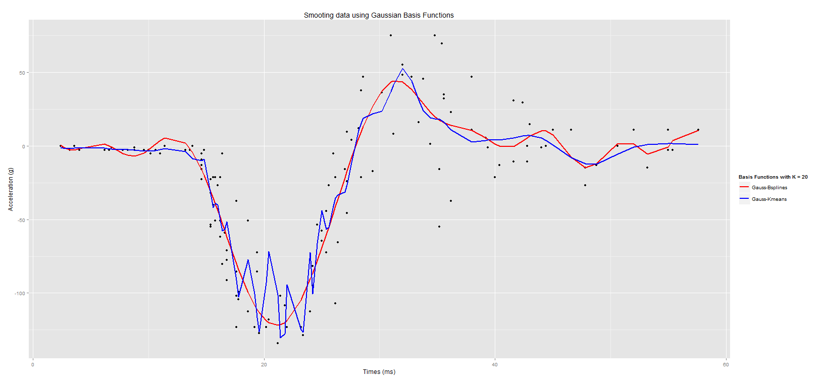
The data I will be using is the motorcycledata from the adlift. The data gives the results of 133 simulations showing the effects of motorcycle crashes on victims heads. I will use 20 basis functions and the hyperparameter will be set to 2 (i.e. \(\nu = 2\)).
In R, this is how it is done.
set.seed(59)
mtt = motorcycledata$time # the timestamps
m = 20 # number of basis functions
nyu = 2 # hyperparameter

##### B-Splines Gaussian basis
range = diff(range(mtt))
kn = seq(min(mtt) - (range/(m-3))*3, max(mtt) + (range/(m-3))*3, by = range/(m-3))
myu = kn[3:(m+2)]
h = diff(kn,lag = 2)/3

BsMotor <- matrix(0,length(mtt),(m))
for (j in 1:m){
  BsMotor[,j] = exp(-0.5*(mtt-myu[j])^2/(h[1]^2))
}

##### K-Means clustering Gaussian basis
k = kmeans(tt, centers = n, algorithm = "Hartigan-Wong")
myu = as.vector(k$centers)
h = k$withinss/k$size

KMotor <- matrix(0, length(mtt), (m))
for (j in 1:m){
  KMotor[,j] = exp(-0.5*(mtt-myu[j])^2/(h[j]*nyu))
}

##### Smoothing Out (using LS)
f1 = function(data, m, B){

  Binv = solve(t(B)%*%B, diag(m))
  S = B%*%Binv%*%t(B)
  return(S%*%data)
}

accel1 = f1(data = motorcycledata$accel,m = m,B = BsMotor)
accel2 = f1(data = motorcycledata$accel,m = m,B = KMotor)

gaussian_motor = setNames(data.frame(motorcycledata[, 2], accel1, accel2), c("Acceleration", "GaussBsplines", "GaussKmeans"))
Here is the output
Concluding comments
As you may have noticed, I used the Least-Square approach to produce the smoothed estimates by multiplying the raw observations by the hat matrix H = \(\Phi (\Phi^{t} \Phi)^{-1} \Phi^{t}\) where \(\Phi\) is the matrix of basis functions. As stated above, the K-means clustering approach underperformed when capturing all the information from the data whereas the B-Splines approach rendered a better fit. Thus far, we have not considered the addition of a penalty term which may help to remediate the rapid fluctuations that we observed when smoothing out our data as well as the choice of the number of basis functions. This will be discussed at a later stage.