In this post we will introduce the Fourier basis functions in the context of Functional Data Analysis. The Fourier basis function is method to smooth out data varying over a continuum and exhibiting a cyclical trend. Smoothing techniques play an important role in Functional Data Analysis (FDA) as they provide insight in the functional behavior of stochastic process. The mathematical background as well as its application will be done. The R-packages used here are: fda and fda.usc. Anyone interested in this topic should check out this website: Functional Data Analysis.
Mathematical Background
For any data analysis in the FDA context, the very first step is to derive the smooth functional data. Let \(t\) be a one-dimensional argument sometimes referred as time. Functions of \(t\) are observed over a discrete grid \(\left\lbrace t_{1},\dots,t_{J} \right\rbrace \in \mathcal{T}\) at sampling values \(t_j\), which may or may not be equally spaced. In order to create a functional datum, a basis needs to be specified. The chosen basis is a linear combination of functions defining the functional object. A functional observation \(X_i\) is defined as follows:
$$X_i(t) \approx \sum_{k=1}^{K} c_{ik}\phi_{k}(t),\text{ }\forall t \in \mathcal{T}$$, where \(\phi_{k}(t)\) (for \(k = 1,\dots,K\)) is the \(k^{th}\) basis function of the expansion and \(c_{ik}\) is the corresponding coefficient. Generally, the observerd data are filled with observational errors (or noise) that are superimposed on the underlying signal. In the real world, we could observed a scenario involving \(N\) processes being observed at the same time. Let \(\mathbf{Y}\) be a vector of \(N\) functional data \(\mathbf{Y} = \left[\mathbf{Y}^T_{1},\dots,\mathbf{Y}^T_{N}\right]^T\), each functional data is written as follows:
$$Y_{ij} = X_{i}(t_{j}) + \epsilon_{ij},\text{ } 1 \leq j \leq J \text{, } 1 \leq i \leq N$$. \(Y_{ij}\) is a noisy observation of the stochastic process \(X_{i}(t_j)\) and \(\epsilon_{ij}\) is a random error with zero mean and variance function \(\sigma^{2}_i\) associated with the \(i^{th}\) functional datum. In vector notation, the \(X_i(t)\) is written as: $$X_{i}(t) \approx \mathbf{c}^{T}_{i}\boldsymbol\phi(t),\text{ }\forall t \in \mathcal{T},\text{ } i = 1,\dots,N$$ where \(\mathbf{c}_{i}\) and \(\mathbf{\phi}(t)\) are \(K\)-vectors.
Fourier Basis
The most appropriate basis for periodic functions defined on an interval \(\mathcal{T}\) is the \(\textit{Fourier Basis}\) where the \(\phi_{k}\)’s take the following form: $$\phi_{o}(t) = 1/\sqrt{|\mathcal{T}|},\; \phi_{2r-1}(t) = \dfrac{sin(r\omega t)}{\sqrt{|\mathcal{T}|/2}} \; \text{and} \; \phi_{2r}(t) = \dfrac{cos(r\omega t)}{\sqrt{|\mathcal{T}|/2}}$$, for \(r=1,\dots,\frac{K-1}{2}\), where \(K\) is the number of basis functions; notice that the \(K\) must be an odd number to compute Fourier Basis. The frequency \(\omega\) determines the period and the length of the interval \(|\mathcal{T}|=2\pi/\omega\).
Practical Application using R
Now we have the necessary theoretical background, it is important to apply it on real data. Let’s consider the Aemet dataset from the R-package fda.usc. It contains daily measurements of Temperature, Wind Speed and Precipitation from \(N = 73\) different weather stations in Spain from 1980 to 2009. For this example, our attention will be on the temperature. In this context, a functional observation consists of 365 pairs \((t_{j},Y_{ij})\) with \(t_{1} = 0.5,\dots,t_{365} = 364.5\) (i.e. \(J = 365\)).
Visualization of Temperature in Oviedo:
suppressPackageStartupMessages(library(fda))
suppressPackageStartupMessages(library(fda.usc))
data(aemet,package = "fda.usc")
tt = aemet$temp$argvals
temp = as.data.frame(aemet$temp$data,row.names=F)
range.tt = aemet$temp$rangeval
inv.temp = data.frame(t(aemet$temp$data)) # 365 x 73 matrix
names(inv.temp) = aemet$df$name # Oviedo is the 10th column of inv.temp
Here is the plot:

Constructing Fourier Basis
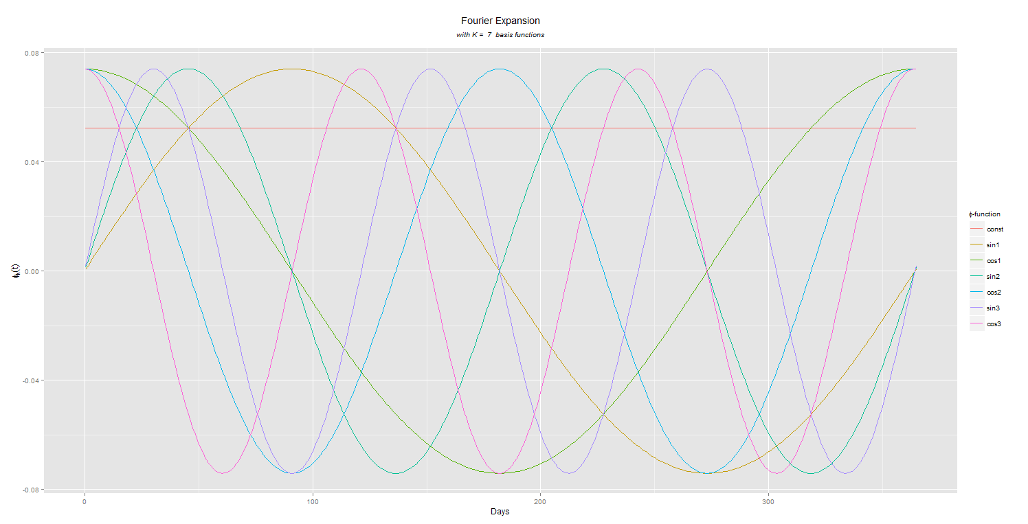
Using the fda package, one can construct a Fourier basis function with create.fourier.basis(rangeval, nbasis) where rangeval is the domain of the \(t\) and nbasis is the number of basis functions applied. Its implementation in R is shown as follow:
temp_k7 = create.fourier.basis(rangeval = range(tt),nbasis = 7)
phimat = eval.basis(tt,basisobj=temp_k7)
phi.frame = data.frame(cbind(phimat,tt))
melt.phi = melt(data=phi.frame,id.vars="tt")
Here is the plot:
Smoothing out
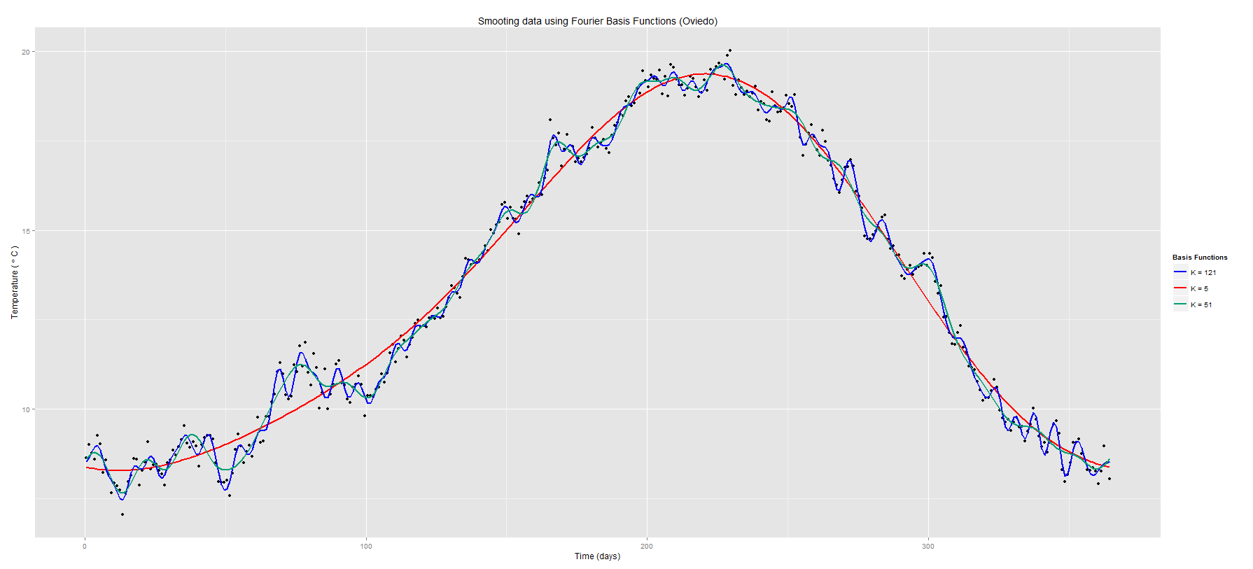
The final step is now to smooth out the daily observations of temperature using our basis functions. We will consider the cases when K, the number of basis functions, is equal to 5, 50 and 121. We construct a functional data object by smoothing data using a roughness penalty with the function smooth.basis(argvals=1:n, y, fdParobj) where argvals is the domain, y is a set of values at discrete sampling points or argument values and fdParobj is the basis function object. In order to evaluate a functional data object at specified argument values, one should use eval.fd(evalarg, fdobj, Lfdobj=0, returnMatrix=FALSE) to convert data to functional object. In R, we get the following:
ovibasis5 = create.fourier.basis(rangeval = range(tt),nbasis = 5)
ovibasis50 = create.fourier.basis(rangeval = range(tt),nbasis = 50)
ovibasis121 = create.fourier.basis(rangeval = range(tt),nbasis = 121)
ovifourier5.fd = smooth.basis(argvals = tt, y = inv.temp[,10],fdParobj = ovibasis5)$fd
ovifourier51.fd = smooth.basis(argvals = tt, y = inv.temp[,10],fdParobj = ovibasis50)$fd
ovifourier121.fd = smooth.basis(argvals = tt, y = inv.temp[,10],fdParobj = ovibasis121)$fd
ovi5 = eval.fd(tt,ovifourier5.fd)
ovi51 = eval.fd(tt,ovifourier51.fd)
ovi121 = eval.fd(tt,ovifourier121.fd)
oviedo = setNames(data.frame(inv.temp[,10],ovi5,ovi51,ovi121),c("Oviedo","Fourier5","Fourier51","Fourier121"))
Here is the plot:
Concluding comments
The result above is telling us that as the number of basis functions is becoming smaller, the curve that we obtain tends to oversmooth the data whereas a large number of basis functions is close to the data points. Fourier Basis are the most appropriate basis for periodic functions defined over an interval \(\mathcal{T}\). The choice of the number of basis functions is usually at the heart of the smoothing exercise, but this will be discussed at a later stage.