Naive Bayes is a supervised machine learning algorithm. As the name implies it’s based on Bayes theorem. In this post, you will discover what’s happening behind the Naive Bayes classifier when you are dealing with continuous predictor variables.
Here I have used R language for coding. Let us see what’s going on behind the scenes in naiveBayes function when the features or predictor variables are continuous in nature.
Understanding Bayes’ theorem
A strong foundation on Bayes theorem as well as Probability functions (density function and distribution function) is essential if you really wanna get an idea of intuitions behind the Naive Bayes algorithm.
Bayes’ theorem is all about finding a probability (we call it posterior probability) based on certain other probabilities which we know in
advance.
As per the theorem,
P(A|B) = P(A) P(B|A)/P(B)
- P(A|B) and P(B|A) are called the conditional probabilities where in P(A|B) means how often A happens given that B happens.
- P(A) and P(B) are called the marginal probabilities which says how likely A or B is on its own (The probability of an event irrespective of the outcomes of other random variables)
P(A/B) is what we are gonna predict, hence called as posterior probability also.
Now in real world we would be having many predictor variables and many class variables. For easy mapping let us call these classes as, C1, C2,…, Ck and the predictor variables (feature vectors) x1,x2,…,xn.
Then using Bayes theorem we would be measuring the conditional probability of an event with a feature vector x1,x2,…,xn belonging to a particular class Ci.
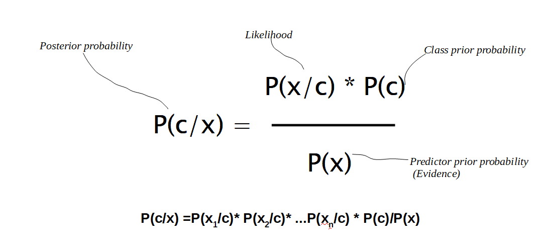
We can formulate the posterior probability P(c|x) from P(c), P(x) and P(x|c) as given below
How probability is calculated in Naive Bayes?
Usually we use the e1071 package to build a Naive Bayes classifier in R. And then using this classifier, we make some predictions on the training data.
So probability for these predictions can be directly calculated based on frequency of occurrences if the features are categorical.
But what if, there are features with continuous values? What the Naive Bayes classifier is actually doing behind the scenes to predict the probabilities of continuous data?
It’s nothing but usage of probability density functions. So here Naive Bayes is generating a Gaussian (Normal) distributions for each predictor variable. The distribution is characterized by two parameters, its mean and standard deviation. Then based on mean and standard deviation of the each predictor variable, the probability for a value to be ‘x’ is calculated using probability density function. (Probability density function gives the probability of observing a measurement with a specific value)
The normal distribution (bell curve) has density
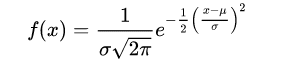
where μ is the mean of the distribution and σ the standard deviation.
f(x) or the probability density function for a value ‘x’ can be calculated using some standard z-table calculations or in R language we have the dnorm function.
So in short once we know the distributions parameters (mean and standard deviation in case of normally distributed data) we can calculate any probability.
dnorm function in R
You can mirror what the naiveBayes function is doing by using dnorm (x, mean=, sd=) function for each class of outcomes. (remember, the class variable is categorical and features can be a mix of continuous and categorical). dnorm in R gives us the probability density function.
dnorm function in R is the back bone of continuous naiveBayes.
Understanding the intuitions behind continuous Naive Bayes – with iris data in R
Let us consider the Iris data in R language.
Iris dataset contains three plant species (setosa,viriginica,versicolor) and four features (Sepal.Length, Sepal.Width, Petal.Length, Petal.Width) measured for each sample.
First we will build the model using Naive Bayes function in e1071 package. And then given a set of features, say Sepal.Length=6.9, Sepal.Width=3.1, Petal.Length=5.0, Petal.Width=2.3 we will predict what would be the species.
So here is the complete code using naiveBayes function for predicting the species.
#Installing e1071 R Package
install.packages(‘e1071’)
library(e1071)
# Read the dataset
data(“iris”)
#studying structure of data
str(iris)
# Partitioning the dataset into training set and test set
split=sample.split(iris,SplitRatio =0.7)
Trainingset=subset(iris,split==TRUE)
Testset=subset(iris,split==FALSE)
# Fitting naïve_bayes model to training Set
install.packages(‘caTools’)
library(‘caTools’)
set.seed(120)
classifier=naiveBayes(x = Trainingset[,-5],
y = Trainingset$Species)
classifier
# Predicting on test data
Y_Pred=predict(classifier,newdata = Testset)
Y_Pred
# Confusion Matrix
cm=table(Testset$Species,Y_Pred)
cm
#Probelm: given a set of features, find to which species that belongs
#defining a new set of data (features) to check the classification
sl=6.9
sw=3.1
pl=5.0
pw=2.3
newfeatures=data.frame(Sepal.Length=sl,Sepal.Width=sw,Petal.Length=pl,Petal.Width=pw)
Y_Pred=predict(classifier,newdata = newfeatures)
Y_Pred
Now on executing the code you can see that the predicted species is Virginica as per naiveBayes function
And now here comes the most interesting part- what’s going on behind the scenes:
We know that Naive Bayes predict the results using probability density functions in the back end.
We are gonna straightaway find out the probabilities using dnorm function for each class variable. The result has to be same as that predicted by naiveBayes function.
For a given set of features,
1. Based on the mean and standard deviation conditional probability would be derived.
2. And then applying Baye’s theorem, probability for each species under the given set of predictor variables would be derived and compared against each other.
3. The one with higher probability would be the predicted result.
Here is the complete code for using prediction by hand (with dnorm function)
install.packages(‘e1071’)
library(e1071)
# Read the dataset
data(“iris”)
#studying structure of data
str(iris)
# Partitioning the dataset into training set and test set
split=sample.split(iris,SplitRatio =0.7)
Trainingset=subset(iris,split==TRUE)
Testset=subset(iris,split==FALSE)
# Fitting naïve_bayes model to training Set
install.packages(‘caTools’)
library(‘caTools’)
set.seed(120)
classifier=naiveBayes(x = Trainingset[,-5],
y = Trainingset$Species)
#Probelm: given a set of features, find to which species that belongs
#defining a new set of data (features) to check the classification
sl=6.9
sw=3.1
pl=5.0
pw=2.3
#Finding Class Prior Probabilities of each species
PriorProb_Setosa= mean(Trainingset$Species==’setosa’)
PriorProb_Virginica= mean(Trainingset$Species==’virginica’)
PriorProb_versicolor= mean(Trainingset$Species==’versicolor’)
#Species wise mean and standard deviation of Sepal Length
#Finding Conditional Probabilities or Likelihood or Prior Probabilities
Setosa= subset(Trainingset, Trainingset$Species==’setosa’)
Virginica= subset(Trainingset, Trainingset$Species==’virginica’)
Versicolor= subset(Trainingset, Trainingset$Species==’versicolor’)
Set=Setosa%>% summarise(mean(Sepal.Length),mean(Sepal.Width),mean(Petal.Length),mean(Petal.Width),
sd(Sepal.Length),sd(Sepal.Width),sd(Petal.Length),sd(Petal.Width))
Vir=Virginica%>% summarise(mean(Sepal.Length),mean(Sepal.Width),mean(Petal.Length),mean(Petal.Width),
sd(Sepal.Length),sd(Sepal.Width),sd(Petal.Length),sd(Petal.Width))
Ver=Versicolor%>% summarise(mean(Sepal.Length),mean(Sepal.Width),mean(Petal.Length),mean(Petal.Width),
sd(Sepal.Length),sd(Sepal.Width),sd(Petal.Length),sd(Petal.Width))
Set_sl=dnorm(sl,mean=Set$`mean(Sepal.Length)`, sd=Set$`sd(Sepal.Length)`)
Set_sw=dnorm(sw,mean=Set$`mean(Sepal.Width)` , sd=Set$`sd(Sepal.Width)`)
Set_pl=dnorm(pl,mean=Set$`mean(Petal.Length)`, sd=Set$`sd(Petal.Length)`)
Set_pw=dnorm(pw,mean=Set$`mean(Petal.Width)` , sd=Set$`sd(Petal.Width)`)
#denominator would be same for all three probabilities. SO we can ignore them in calculations
ProbabilitytobeSetosa =Set_sl*Set_sw*Set_pl*Set_pw*PriorProb_Setosa
Vir_sl=dnorm(sl,mean=Vir$`mean(Sepal.Length)`, sd=Vir$`sd(Sepal.Length)`)
Vir_sw=dnorm(sw,mean=Vir$`mean(Sepal.Width)` , sd=Vir$`sd(Sepal.Width)`)
Vir_pl=dnorm(pl,mean=Vir$`mean(Petal.Length)`, sd=Vir$`sd(Petal.Length)`)
Vir_pw=dnorm(pw,mean=Vir$`mean(Petal.Width)` , sd=Vir$`sd(Petal.Width)`)
ProbabilitytobeVirginica =Vir_sl*Vir_sw*Vir_pl*Vir_pw*PriorProb_Virginica
Ver_sl=dnorm(sl,mean=Ver$`mean(Sepal.Length)`, sd=Ver$`sd(Sepal.Length)`)
Ver_sw=dnorm(sw,mean=Ver$`mean(Sepal.Width)` , sd=Ver$`sd(Sepal.Width)`)
Ver_pl=dnorm(pl,mean=Ver$`mean(Petal.Length)`, sd=Ver$`sd(Petal.Length)`)
Ver_pw=dnorm(pw,mean=Ver$`mean(Petal.Width)` , sd=Ver$`sd(Petal.Width)`)
ProbabilitytobeVersicolor=Ver_sl*Ver_sw*Ver_pl*Ver_pw*PriorProb_versicolor
ProbabilitytobeSetosa
ProbabilitytobeVirginica
ProbabilitytobeVersicolor
On executing this code, you can see that the probability to be Virginica is higher than that of other two. And this implies that the given set of features belong to the class Virginica. And the same results were predicted using naiveBayes function.
A-priori probabilities and conditional probabilities
When you run the scripts in R for the continuous / numeric variables, you might have seen tables titled A-priori probabilities and conditional probabilities. A screenshot from console is given below
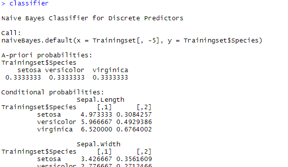
The table titled A-priori probabilities gives prior probability for each class (P(c)) in your training set. This gives the class distribution in the data(‘A priori’ is Latin for ‘from before’) which can be straight away calculated based on the number of occurrences as below,
P(c) = n(c)/n(S), where, P(c) is the probability of an event “c” n(c) is the number of favorable outcomes. n(S) is the total number of events in the sample space.
The given table of conditional probabilities is not showing the probabilities, but the distribution parameters (or rather the mean and standard deviation of the continuous data). Remember, if features were categorical, this table would be indicating the probability value itself.
Some Additional points to keep in mind
- Rather than calculating the tables by hand you may just use the naiveBayes results itself
Here in the above script using dnorm, I have calculated mean and standard deviation by hand. Instead you can derive it using a simple code.
For example if you want to see the mean and standard deviation of sepal length for each species, just run this
>classifier$tables$Sepal.Length - Dropping the denominator (p(x)) probabilities in calculations
Have you noticed that I have dropped the denominator value in probability calculations?
Because the denominator (p(x)) would be same for all when we compare the probabilities for each class under the specified features. So we can just get rid of that. We just need to compare the top parts of the calculation. Also keep in mind that we are comparing the probabilities only and hence omitted the denominator. If we need to get the actual probability value, denominator shouldn’t be omitted. - What if the continuous data is not normally distributed?
There are of course other distributions like Bernoulli, multinomial etc, and not just Gausian distribution alone. But the logic behind all is the same: assuming the feature satisfies a certain distribution, estimating the parameters of the distribution, and then getting the probability density function. - Kernel based densities
Kernel based densities may perform better when continuous variables are not normally distributed. It might improve the test accuracy rate. While making the model input this code ‘useKernel=T’ - Discretization strategy for continuous Naivebayes
For predicting the class-conditional probabilities for continuous attributes in naive Bayes classifiers we can use a disretization strategy also. Discretization works by breaking the data into categorical values. This approach which transforms the continuous attributes into ordinal attributes is not covered in this article at present. - Why Naivebayes is called Naive?
The Naive Bayes algorithm is called “Naive” because it makes the assumption that the occurrence of a certain feature is independent of the occurrence of other features while in reality, they may be dependent in some way!