Understanding the Covariance Matrix

This article is showing a geometric and intuitive explanation of the covariance matrix and the way it describes the shape of a data set. We will describe the geometric relationship of the covariance matrix with the use of linear transformations and eigendecomposition.

Introduction

Before we get started, we shall take a quick look at the difference between covariance and variance. Variance measures the variation of a single random variable (like the height of a person in a population), whereas covariance is a measure of how much two random variables vary together (like the height of a person and the weight of a person in a population). The formula for variance is given by

$$
\sigma^2_x = \frac{1}{n-1} \sum^{n}_{i=1}(x_i – \bar{x})^2 \\
$$

where \(n\) is the number of samples (e.g. the number of people) and \(\bar{x}\) is the mean of the random variable \(x\) (represented as a vector). The covariance \(\sigma(x, y)\) of two random variables \(x\) and \(y\) is given by

$$
\sigma(x, y) = \frac{1}{n-1} \sum^{n}_{i=1}{(x_i-\bar{x})(y_i-\bar{y})}
$$

with n samples. The variance \(\sigma_x^2\) of a random variable \(x\) can be also expressed as the covariance with itself by \(\sigma(x, x)\).

Covariance Matrix

With the covariance we can calculate entries of the covariance matrix, which is a square matrix given by \(C_{i,j} = \sigma(x_i, x_j)\) where \(C \in \mathbb{R}^{d \times d}\) and \(d\) describes the dimension or number of random variables of the data (e.g. the number of features like height, width, weight, …). Also the covariance matrix is symmetric since \(\sigma(x_i, x_j) = \sigma(x_j, x_i)\). The diagonal entries of the covariance matrix are the variances and the other entries are the covariances. For this reason, the covariance matrix is sometimes called the _variance-covariance matrix_. The calculation for the covariance matrix can be also expressed as

$$
C = \frac{1}{n-1} \sum^{n}_{i=1}{(X_i-\bar{X})(X_i-\bar{X})^T}
$$

where our data set is expressed by the matrix \(X \in \mathbb{R}^{n \times d}\). Following from this equation, the covariance matrix can be computed for a data set with zero mean with \( C = \frac{XX^T}{n-1}\) by using the semi-definite matrix \(XX^T\).

In this article, we will focus on the two-dimensional case, but it can be easily generalized to more dimensional data. Following from the previous equations the covariance matrix for two dimensions is given by

$$
C = \left( \begin{array}{ccc}
\sigma(x, x) & \sigma(x, y) \\
\sigma(y, x) & \sigma(y, y) \end{array} \right)
$$

We want to show how linear transformations affect the data set and in result the covariance matrix. First we will generate random points with mean values \(\bar{x}\), \(\bar{y}\) at the origin and unit variance \(\sigma^2_x = \sigma^2_y = 1\) which is also called white noise and has the identity matrix as the covariance matrix.

import numpy as np
import matplotlib.pyplot as plt
%matplotlib inline

plt.style.use('ggplot')
plt.rcParams['figure.figsize'] = (12, 8)

# Normal distributed x and y vector with mean 0 and standard deviation 1
x = np.random.normal(0, 1, 500)
y = np.random.normal(0, 1, 500)
X = np.vstack((x, y)).T

plt.scatter(X[:, 0], X[:, 1])
plt.title('Generated Data')
plt.axis('equal');

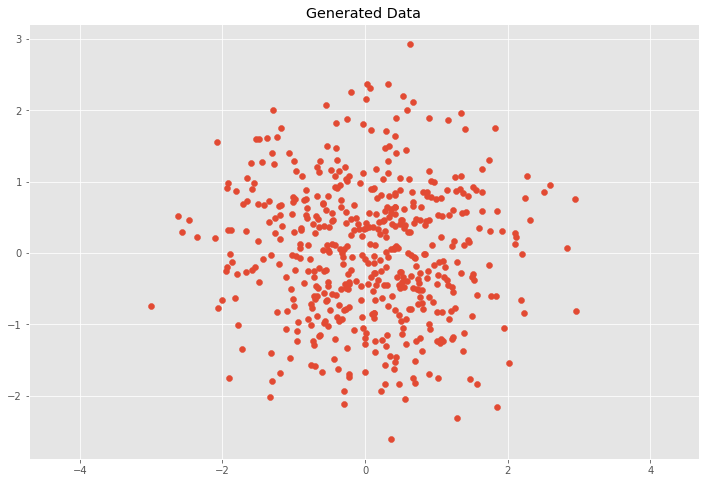
This case would mean that \(x\) and \(y\) are independent (or uncorrelated) and the covariance matrix \(C\) is

$$
C = \left( \begin{array}{ccc}
\sigma_x^2 & 0 \\
0 & \sigma_y^2 \end{array} \right)
$$

We can check this by calculating the covariance matrix

# Covariance
def cov(x, y):
    xbar, ybar = x.mean(), y.mean()
    return np.sum((x - xbar)*(y - ybar))/(len(x) - 1)

# Covariance matrix
def cov_mat(X):
    return np.array([[cov(X[0], X[0]), cov(X[0], X[1])], \
                     [cov(X[1], X[0]), cov(X[1], X[1])]])

# Calculate covariance matrix 
cov_mat(X.T) # (or with np.cov(X.T))
array([[ 1.008072  , -0.01495206],
       [-0.01495206,  0.92558318]])

Which approximatelly gives us our expected covariance matrix with variances \(\sigma_x^2 = \sigma_y^2 = 1\).

Linear Transformations of the Data Set

Next, we will look at how transformations affect our data and the covariance matrix \(C\). We will transform our data with the following scaling matrix.

$$
S = \left( \begin{array}{ccc}
s_x & 0 \\
0 & s_y \end{array} \right)
$$

where the transformation simply scales the \(x\) and \(y\) components by multiplying them by \(s_x\) and \(s_y\) respectively. What we expect is that the covariance matrix \(C\) of our transformed data set will simply be

$$
C = \left( \begin{array}{ccc}
(s_x\sigma_x)^2 & 0 \\
0 & (s_y\sigma_y)^2 \end{array} \right)
$$

which means that we can extract the scaling matrix from our covariance matrix by calculating \(S = \sqrt{C}\) and the data is transformed by \(Y = SX\).

# Center the matrix at the origin
X = X - np.mean(X, 0)

# Scaling matrix
sx, sy = 0.7, 3.4
Scale = np.array([[sx, 0], [0, sy]])

# Apply scaling matrix to X
Y = X.dot(Scale)

plt.scatter(Y[:, 0], Y[:, 1])
plt.title('Transformed Data')
plt.axis('equal')

# Calculate covariance matrix
cov_mat(Y.T)
array([[ 0.50558298, -0.09532611],
       [-0.09532611, 10.43067155]])

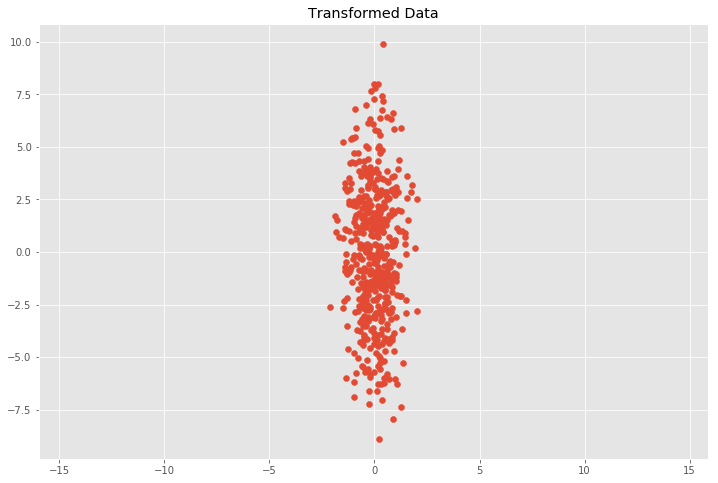
We can see that this does in fact approximately match our expectation with \(0.7^2 = 0.49\) and \(3.4^2 = 11.56\) for \((s_x\sigma_x)^2\) and \((s_y\sigma_y)^2\). This relation holds when the data is scaled in \(x\) and \(y\) direction, but it gets more involved for other linear transformations.

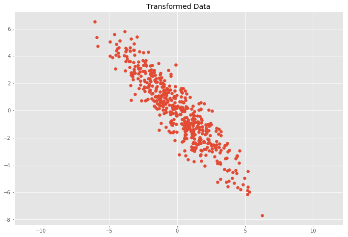
Now we will apply a linear transformation in the form of a transformation matrix \(T\) to the data set which will be composed of a two dimensional rotation matrix \(R\) and the previous scaling matrix \(S\) as follows

$$T = RS$$

where the rotation matrix \(R\) is given by

$$
R = \left( \begin{array}{ccc}
cos(\theta) & -sin(\theta) \\
sin(\theta) & cos(\theta) \end{array} \right)
$$

where \(\theta\) is the rotation angle. The transformed data is then calculated by \(Y = TX\) or \(Y = RSX\).

# Scaling matrix
sx, sy = 0.7, 3.4
Scale = np.array([[sx, 0], [0, sy]])

# Rotation matrix
theta = 0.77*np.pi
c, s = np.cos(theta), np.sin(theta)
Rot = np.array([[c, -s], [s, c]])

# Transformation matrix
T = Scale.dot(Rot)

# Apply transformation matrix to X
Y = X.dot(T)

plt.scatter(Y[:, 0], Y[:, 1])
plt.title('Transformed Data')
plt.axis('equal');

# Calculate covariance matrix
cov_mat(Y.T)
array([[ 4.94072998, -4.93536067],
       [-4.93536067,  5.99552455]])

This leads to the question of how to decompose the covariance matrix \(C\) into a rotation matrix \(R\) and a scaling matrix \(S\).

Eigen Decomposition of the Covariance Matrix

Eigen Decomposition is one connection between a linear transformation and the covariance matrix. An eigenvector is a vector whose direction remains unchanged when a linear transformation is applied to it. It can be expressed as

$$ Av=\lambda v $$

where \(v\) is an eigenvector of \(A\) and \(\lambda\) is the corresponding eigenvalue. If we put all eigenvectors into the columns of a Matrix \(V\) and all eigenvalues as the entries of a diagonal matrix \(L\) we can write for our covariance matrix \(C\) the following equation

$$ CV = VL $$

where the covariance matrix can be represented as

$$ C = VLV^{-1} $$

which can be also obtained by Singular Value Decomposition. The eigenvectors are unit vectors representing the direction of the largest variance of the data, while the eigenvalues represent the magnitude of this variance in the corresponding directions. This means \(V\) represents a rotation matrix and \(\sqrt{L}\) represents a scaling matrix. From this equation, we can represent the covariance matrix \(C\) as

$$ C = RSSR^{-1} $$

where the rotation matrix \(R=V\) and the scaling matrix \(S=\sqrt{L}\). From the previous linear transformation \(T=RS\) we can derive

$$ C = RSSR^{-1} = TT^T $$

because \(T^T = (RS)^T=S^TR^T = SR^{-1}\) due to the properties \(R^{-1}=R^T\) since \(R\) is orthogonal and \(S = S^T\) since \(S\) is a diagonal matrix. This enables us to calculate the covariance matrix from a linear transformation. In order to calculate the linear transformation of the covariance matrix, one must calculate the eigenvectors and eigenvectors from the covariance matrix \(C\). This can be done by calculating

$$ T = V\sqrt{L} $$

where \(V\) is the previous matrix where the columns are the eigenvectors of \(C\) and \(L\) is the previous diagonal matrix consisting of the corresponding eigenvalues. The transformation matrix can be also computed by the Cholesky decomposition with \(Z = L^{-1}(X-\bar{X})\) where \(L\) is the Cholesky factor of \(C = LL^T\).

We can see the basis vectors of the transformation matrix by showing each eigenvector \(v\) multiplied by \(\sigma = \sqrt{\lambda}\). By multiplying \(\sigma\) with 3 we cover approximately \(99.7\%\) of the points according to the three sigma rule if we would draw an ellipse with the two basis vectors and count the points inside the ellipse.

C = cov_mat(Y.T)
eVe, eVa = np.linalg.eig(C)

plt.scatter(Y[:, 0], Y[:, 1])
for e, v in zip(eVe, eVa.T):
    plt.plot([0, 3*np.sqrt(e)*v[0]], [0, 3*np.sqrt(e)*v[1]], 'k-', lw=2)
plt.title('Transformed Data')
plt.axis('equal');

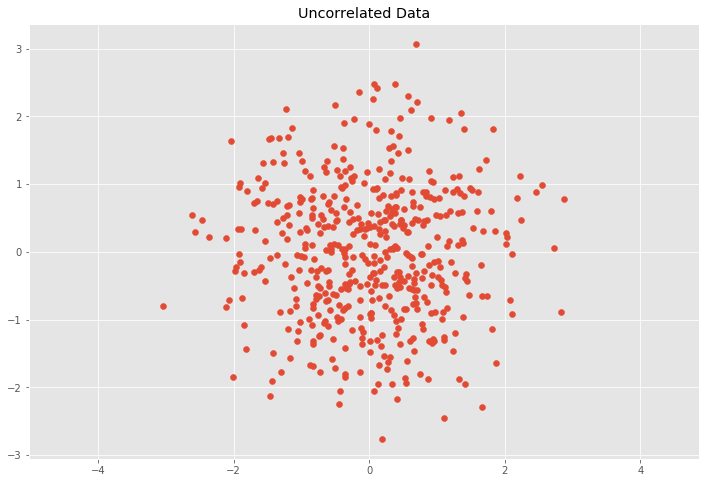
We can now get from the covariance the transformation matrix \(T\) and we can use the inverse of \(T\) to remove correlation (whiten) the data.

C = cov_mat(Y.T)

# Calculate eigenvalues
eVa, eVe = np.linalg.eig(C)

# Calculate transformation matrix from eigen decomposition
R, S = eVe, np.diag(np.sqrt(eVa))
T = R.dot(S).T

# Transform data with inverse transformation matrix T^-1
Z = Y.dot(np.linalg.inv(T))

plt.scatter(Z[:, 0], Z[:, 1])
plt.title('Uncorrelated Data')
plt.axis('equal');

# Covariance matrix of the uncorrelated data
cov_mat(Z.T)
array([[ 1.00000000e+00, -1.24594167e-16],
       [-1.24594167e-16,  1.00000000e+00]])

An interesting use of the covariance matrix is in the Mahalanobis distance, which is used when measuring multivariate distances with covariance. It does that by calculating the uncorrelated distance between a point \(x\) to a multivariate normal distribution with the following formula

$$ D_M(x) = \sqrt{(x – \mu)^TC^{-1}(x – \mu))} $$

where \(\mu\) is the mean and \(C\) is the covariance of the multivariate normal distribution (the set of points assumed to be normal distributed). A derivation of the Mahalanobis distance with the use of the Cholesky decomposition can be found in this article.

Conclusion

In this article we saw the relationship of the covariance matrix with linear transformation which is an important building block for understanding and using PCA, SVD, the Bayes Classifier, the Mahalanobis distance and other topics in statistics and pattern recognition. I found the covariance matrix to be a helpful cornerstone in the understanding of the many concepts and methods in pattern recognition and statistics.

Many of the matrix identities can be found in The Matrix Cookbook. The relationship between SVD, PCA and the covariance matrix are elegantly shown in this question.