I was working on monthly power demand in the Telangana state of India and used Holt-Winters methodology using R to arrive at prediction forecasts. The data is since June 2014 from CEA website for Telangana (the state was formed in June 2014), so, data is available from that time only. I have listed my findings and would like your review/feedback on this.
Load the required library packages.
library(readxl)
require(graphics)
library(forecast)
library(timeSeries)
library (tseries)
library(ggplot2)
library(TTR)
I extracted the data from June 2014 until May 2017 and stored it in Telangana_Power.
Create Time series object for power requirement in Telangana
The Time series object can be created using ts()function. As we have data starting June 2014, we have kept it as starting point.
TS_Power_Req <- ts(Telangana_Power$Requirement..MU., start = c(2014, 6), frequency = 12)
head(TS_Power_Req)
  Jun Jul Aug Sep Oct Nov
2014 3830 4354 4847 4442 4900 3912
Graph for Power requirement trend in Telangana since June 2014

We can see from above time series plot that there seems to be seasonal variation in power demand per month: there is a peak for April, August and October and a trough every June.
The dip in September may be attributed to Agricultural demand drops down due to cutting season for the crops sown in June. The spikes in August, October and Jan are all due to agricultural season activity.
Again, it seems that this time series could probably be described using an additive model, as the seasonal fluctuations are roughly constant in size over time and do not seem to depend on the level of the time series, and the random fluctuations also seem to be roughly constant in size over time.
Visualize the Power requirement for Telangana by decomposing the time series
A seasonal time series consists of a trend component, a seasonal component and an irregular component. Decomposing the time series means separating the time series into these three components: that is, estimating these three components. To estimate the trend component and seasonal component of a seasonal time series that can be described using an additive model, we can use the decompose() function in R. This function estimates the trend, seasonal, and irregular components of a time series that can be described using an additive model. The function decompose() returns a list object as its result, where the estimates of the seasonal component, trend component and irregular component are stored in named elements of that list objects, called “seasonal”, “trend”, and “random” respectively.
TS_Power_STL <- decompose(TS_Power_Req)
The estimated values of the seasonal, trend and irregular components are now stored in variables TS_Power_STL$seasonal, TS_Power_STL$trend and TS_Power_STL$random. We can print out the estimated values of the seasonal component by typing:
TS_Power_STL$seasonal
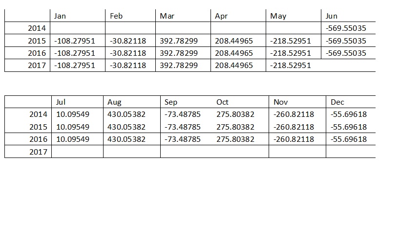
The estimated seasonal factors are given for the duration Jun 2014-May 2017, and are the same for each year. The largest seasonal factor is for March (392.78) and August (430.05), and the lowest is for June (-569.55), indicating that there seems to be a peak demand in August and a trough in births in June each year.
The estimated trend, seasonal, and irregular components of the time series can be plotted by using the plot() function :
plot(TS_Power_STL, col = "steelblue")
Gives this plot:

The plot above shows the original time series (top), the estimated trend component (second from top), the estimated seasonal component (third from top), and the estimated irregular component (bottom). We see that the estimated trend component shows a steady decrease from 2014 to 2015, followed by low constant demand and then a sharp increase in 2016 and thereafter.
Seasonally Adjusting
For seasonal time series that can be described using an additive model, we have to seasonally adjust the time series by estimating the seasonal component and subtracting the estimated seasonal component from the original time series. We can do this using the estimate of the seasonal component calculated by the decompose() function.
To seasonally adjust the time series, we can estimate the seasonal component using decompose(), and then subtract the seasonal component from the original time series:
TS_Power_Seasonally_adjusted <- TS_Power_Req - TS_Power_STL$seasonal
We can then plot the seasonally adjusted time series using the plot() function, by typing:
plot(TS_Power_Seasonally_adjusted)
Gives this plot:
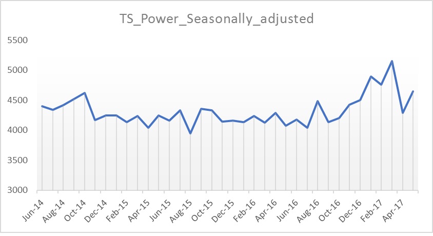
As can be seen, the seasonal variation has been removed from the seasonally adjusted time series. The seasonally adjusted time series now just contains the trend component and an irregular component.
Check for Stationarity
A stationary time series is one whose properties do not depend on the time at which the series is observed. So, time series with trends, or with seasonality, are not stationary — the trend and seasonality will affect the value of the time series at different times. On the other hand, a white noise series is stationary — it does not matter when it is observed, it should look much the same at any period of time. The augmented Dickey-Fuller (ADF) test is a formal statistical test for stationarity. The null hypothesis assumes that the series is non-stationary. So, large p-values are indicative of non-stationarity, and small p-values suggest stationarity. ADF procedure tests whether the change in Y can be explained by lagged value and a linear trend. If the contribution of the lagged value to the change in Y is non-significant and there is a presence of a trend component, the series is non-stationary and null hypothesis will not be rejected.
adf.test(TS_Power_Req, alternative = "stationary")
     Augmented Dickey-Fuller Test
data: TS_Power_Req
Dickey-Fuller = -3.0841, Lag order = 3, p-value = 0.1513
alternative hypothesis: stationary
The high P-value (>0.05) indicates that our data is non-stationary, the power demand changes through time, A formal ADF test does not reject the null hypothesis of non-stationarity, confirming our visual inspection.
As confirmed by using decompose() function and ADF unit test that Power demand data is non-stationary, we will first use Holt-Winters.
Holt-Winters Exponential Smoothing and Forecast prediction
We have a time series data that can be described using an additive model with varying (decreases then increases) trend and seasonality. The random fluctuations in the data are roughly constant in size over time. Hence, we can use Holt-Winters exponential smoothing to make short-term forecasts. Holt-Winters exponential smoothing estimates the level, slope and seasonal component at the current time point. Smoothing is controlled by three parameters: alpha, beta, and gamma, for the estimates of the level, slope b of the trend component, and the seasonal component, respectively, at the current time point. The parameters alpha, beta, and gamma all have values between 0 and 1, and values that are close to 0 mean that relatively little weight is placed on the most recent observations when making forecasts of future values. To make forecasts, we can fit a predictive model using the HoltWinters() function.
TS_Power_Req_Forecast <- HoltWinters(TS_Power_Req)
TS_Power_Req_Forecast
Holt-Winters exponential smoothing with trend and additive seasonal component.
Call:
HoltWinters(x = TS_Power_Req)
Smoothing parameters:
 alpha: 0.4249225
 beta : 0
 gamma: 0

Coefficients:
          [,1]
a  4641.375897
b    -8.990676
s1 -589.194444
s2  173.597222
s3  205.638889
s4  115.055556
s5  434.388889
s6 -293.736111
s7  -84.819444
s8 -127.444444
s9 -138.486111
s10 412.597222
s11  49.138889
s12 -156.736111
TS_Power_Req_Forecast$SSE
[1] 1877460
The estimated values of alpha, beta and gamma are 0.42, 0.00, and 0.00, respectively. The value of alpha (0.42) is relatively low, indicating that the estimate of the level at the current time point is based upon both recent observations and some observations in the more distant past. The value of beta is 0.00, indicating that the estimate of the slope b of the trend component is not updated over the time series, and instead is set equal to its initial value. This makes good intuitive sense, as the level changes quite a bit over the time series, but the slope b of the trend component remains roughly the same. Finally, the value of gamma (0.00) is least, indicating that the estimate of the seasonal component at the current time point is just based upon old observations.
We can plot the original time series as a black line, with the forecasted values as a red line on top of that:
plot(TS_Power_Req_Forecast)
Gives this plot:
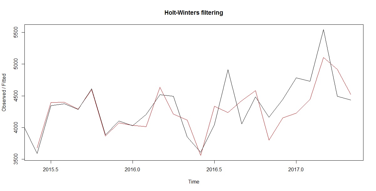
We see from the plot that the Holt-Winters exponential method is very successful in predicting the seasonal peaks, which occur roughly in March and August every year.
To make forecasts for future times not included in the original time series, we use the “forecast()” function in the forecast package.
Predicting the demand for next 6 months based on Holt-Winter methodology.
TS_Power_Demand_Future <- forecast(TS_Power_Req_Forecast, h = 6,
                                              level = c(85,0.95))
# Future demand table
TS_Power_Demand_Future
        Point Forecast   Lo 85   Hi 85 Lo 0.95 Hi 0.95
Jun 2017      4043.191 3640.440 4445.942 4039.860 4046.522
Jul 2017      4796.992 4359.389 5234.595 4793.372 4800.611
Aug 2017      4820.043 4350.166 5289.920 4816.156 4823.929
Sep 2017      4720.469 4220.396 5220.542 4716.333 4724.605
Oct 2017      5030.811 4502.265 5559.358 5026.440 5035.183
Nov 2017      4293.696 3738.134 4849.258 4289.101 4298.291
Let us visualize the future demand forecast.
plot(TS_Power_Demand_Future,ylab="Power Demand in Telangana (MU)",
    plot.conf=FALSE, type="o", fcol="white", xlab="Year")x``
lines(fitted(TS_Power_Demand_Future), col="red", lty=2)
lines(TS_Power_Demand_Future$mean, type="o", col="red")
legend("topleft",lty=1, pch=0.5, col=1:3,
      c("TS Power Requirement Original Data","Holt Winters' Methodology Additive"))
Gives this plot:
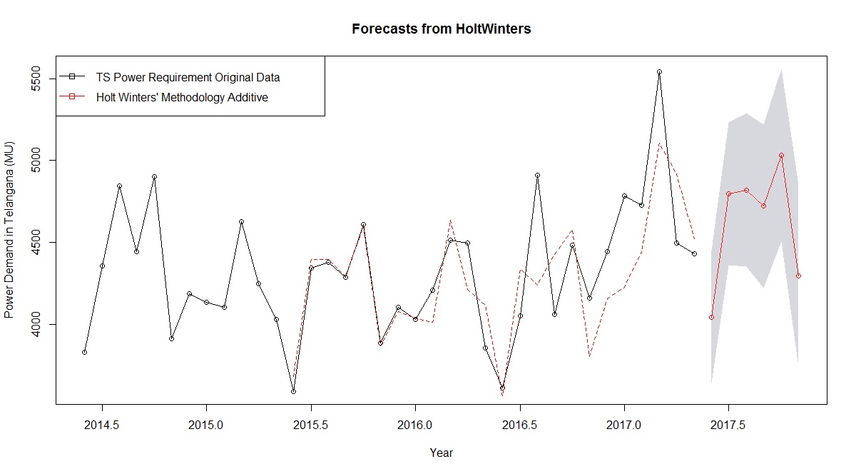
The forecasts are shown as a red line, and the shaded areas show 85% and 95% prediction intervals, respectively.
-
Note: The real values of forecasts are available on CEA site for the month of June 17. The power demand requirement value for Telangana is 3877(MU). The forecast figures are 4043. The % deviation of forecast value from original data (June 17) is therefore [(4043-3877/3877)*100%] = 4.28 %. For the month of July, the power demand requirement value for Telangana was 4896 (MU). The forecasted figures by our model is 4796. The % deviation of forecasted value from original data (July 17) is therefore [(4896-4796/4896)*100%] = 2.04 %. This looks like very close and good estimate.
Future forecast figures from our model are:
- Months Point Forecast Lo 85 Hi 85 Lo 0.95 Hi 0.95
Aug 2017 4820.043 4350.166 5289.920 4816.156 4823.929
Sep 2017 4720.469 4220.396 5220.542 4716.333 4724.605
Oct 2017 5030.811 4502.265 5559.358 5026.440 5035.183
Nov 2017 4293.696 3738.134 4849.258 4289.101 4298.291
Forecast – Errors
The ‘forecast errors’ are calculated as the observed values minus predicted values, for each time point. We can only calculate the forecast errors for the time period covered by our original time series, which is 2015-2017 for the rainfall data. One measure of the accuracy of the predictive model is the sum-of-squared-errors (SSE) for the in-sample forecast errors.
The in-sample forecast errors are stored in the named element “residuals” of the list variable returned by forecast.HoltWinters(). If the predictive model cannot be improved upon, there should be no correlations between forecast errors for successive predictions.
To figure out whether this is the case, we can obtain a correlogram of the in-sample forecast errors using the acf() function and carrying out the Ljung-Box test.
acf(TS_Power_Demand_Future$residuals, lag.max=20, na.action = na.contiguous)
Gives this plot:

We can see from the sample correlogram that the autocorrelation is away from touching the significance bounds. Still, to test whether there is significant evidence for non-zero correlations at lags 1-20, we can carry out a Ljung-Box test.
Box.test(TS_Power_Demand_Future$residuals, lag=20, type="Ljung-Box")
    Box-Ljung test
data: TS_Power_Demand_Future$residuals
X-squared = 12.099, df = 20, p-value = 0.9126
Here the Ljung-Box test statistic is 12 and the p-value is 0.9, so there is little evidence of non-zero autocorrelations in the in-sample forecast errors at lags 1-20.
Also, Model Accuracy using accuracy() is:
accuracy(TS_Power_Demand_Future)
                  ME    RMSE     MAE     MPE    MAPE     MASE      ACF1
Training set 56.68015 279.6918 208.5326 1.013863 4.654729 0.7455357 -0.1541972
The errors look within range.
If you have question leave a comment below.