Use of receiver operator curves (ROC) for binary outcome logistic regression is well known. However, the outcome of interest in epidemiological studies are often time-to-event outcomes. Using time-dependent ROC that changes over time may give a fuller description of prediction models in this setting.
Time-dependent ROC definitions
Let \(M_{i}\) be a baseline (time 0) scalar marker that is used for mortality prediction. Its prediction performance is dependent on time of assessment t when the outcome is observed over time. Intuitively, the marker value measured at time zero should become less relevant as time passes by. Thus, the prediction performance (discrimination) measured by ROC is a function of time t. There are several definitions. I examine two of them here. The notation follows Heagerty et al (2005).1
Cumulative case/dynamic control ROC
The cumulative case/dynamic control ROC2 defines sensitivity and specificity at time t at a threshold c as follows.
\begin{align*}
\text{sensitivity}^{\mathbb{C}}(c,t) &= P(M_{i} > c | T_{i} \le t)\\
\text{specificity}^{\mathbb{D}}(c,t) &= P(M_{i} \le c | T_{i} > t)\\
\end{align*}
The cumulative sensitivity considers those who have died by time t as the denominator (disease) and those who have a marker value higher than c among them as true positives (positive in disease). The dynamic specificity regards those who are still alive at time t as the denominator (health) and those who have a marker value less than or equal to c among them as true negatives (negative in health). Varying the threshold value c from the lowest value to the highest value gives the entire ROC curve at time t. The definitions are based on the latent event time \(T_{i}\), which is not observed for censored individuals. Estimation must account for censoring.2 This is one gives the prediction performance for the risk (cumulative incidence) of events over the t-year period.
Incident case/dynamic control ROC
The incident case/dynamic control ROC1 defines sensitivity and specificity at time t at a threshold c as follows.
\begin{align*}
\text{sensitivity}^{\mathbb{I}}(c,t) &= P(M_{i} > c | T_{i} = t)\\
\text{specificity}^{\mathbb{D}}(c,t) &= P(M_{i} \le c | T_{i} > t)\\
\end{align*}
The cumulative sensitivity considers those who die at time t as the denominator (disease) and those who have a marker value higher than c among them as true positives (positive in disease). The dynamic specificity does not change. This definition partition the risk set at time t (those who have \(T_{i} \ge t\)) into cases and controls. Censoring seems less problematic with this approach under the non-informative censoring assumption. This one gives the prediction performance for the hazard (incidence in the risk set) of events at t-year among those who are in the risk set at t.
Time-dependent ROC R implementation
Data preparation
We use the ovarian dataset3 in the survival package as an example. The time-to-event outcome is time-to-death. The Kaplan-Meier plot is the following.
## Note the MASS package masks select()!
library(tidyverse)
## https://github.com/tidyverse/tibble/issues/395
options(crayon.enabled = FALSE)
## Used for the dataset.
library(survival)
## Used for visualizaiton.
library(survminer)
## Load the Ovarian Cancer Survival Data
data(ovarian)
## Turn into a data_frame
ovarian <- as_data_frame(ovarian)
## Plot
ggsurvplot(survfit(Surv(futime, fustat) ~ 1,
                   data = ovarian),
           risk.table = TRUE,
           break.time.by = 180)
Gives this plot:
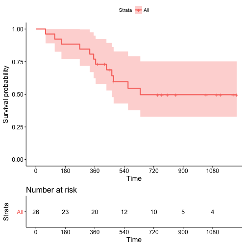
No events occurred beyond 720 days in the dataset.
We fit a Cox regression model using all the covariates and construct a risk score based on the linear predictor.
## Fit a Cox model
coxph1 <- coxph(formula = Surv(futime, fustat) ~ pspline(age, df = 4) + factor(resid.ds) +
                    factor(rx) + factor(ecog.ps),
                data    = ovarian)
## Obtain the linear predictor
ovarian$lp <- predict(coxph1, type = "lp")
ovarian
# A tibble: 26 x 7
   futime fustat   age resid.ds    rx ecog.ps      lp
 *  <dbl>  <dbl> <dbl>    <dbl> <dbl>   <dbl>   <dbl>
 1     59      1  72.3        2     1       1  3.48
 2    115      1  74.5        2     1       1  3.35
 3    156      1  66.5        2     1       2  2.88
 4    421      0  53.4        2     2       1 -0.299
 5    431      1  50.3        2     1       1  0.301
 6    448      0  56.4        1     1       2 -0.304
 7    464      1  56.9        2     2       2  0.0875
 8    475      1  59.9        2     2       2  0.121
 9    477      0  64.2        2     1       1  1.17
10    563      1  55.2        1     2       2 -0.666
# ... with 16 more rows
Cumulative case/dynamic control ROC
The survivalROC package implements the cumulative case/dynamic control ROC.2
library(survivalROC)
## Define a helper functio nto evaluate at various t
survivalROC_helper <- function(t) {
    survivalROC(Stime        = ovarian$futime,
                status       = ovarian$fustat,
                marker       = ovarian$lp,
                predict.time = t,
                method       = "NNE",
                span = 0.25 * nrow(ovarian)^(-0.20))
}
## Evaluate every 180 days
survivalROC_data <- data_frame(t = 180 * c(1,2,3,4,5,6)) %>%
    mutate(survivalROC = map(t, survivalROC_helper),
           ## Extract scalar AUC
           auc = map_dbl(survivalROC, magrittr::extract2, "AUC"),
           ## Put cut off dependent values in a data_frame
           df_survivalROC = map(survivalROC, function(obj) {
               as_data_frame(obj[c("cut.values","TP","FP")])
           })) %>%
    dplyr::select(-survivalROC) %>%
    unnest() %>%
    arrange(t, FP, TP)
## Plot
survivalROC_data %>%
    ggplot(mapping = aes(x = FP, y = TP)) +
    geom_point() +
    geom_line() +
    geom_label(data = survivalROC_data %>% dplyr::select(t,auc) %>% unique,
               mapping = aes(label = sprintf("%.3f", auc)), x = 0.5, y = 0.5) +
    facet_wrap( ~ t) +
    theme_bw() +
    theme(axis.text.x = element_text(angle = 90, vjust = 0.5),
          legend.key = element_blank(),
          plot.title = element_text(hjust = 0.5),
          strip.background = element_blank())
Gives this plot:
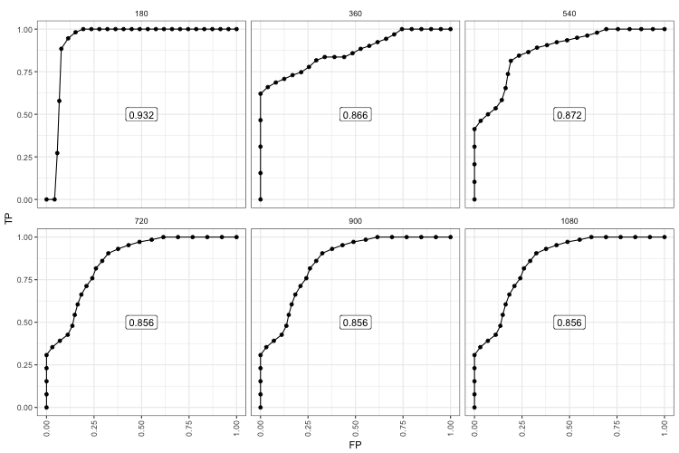
The 180-day ROC looks the best. However, this is because there were very few events up until this point. After the last observed event (\(t \ge 720\)) the AUC stabilized at 0.856. The performance does not decay because the individuals with high risk score who did die keep contributing to the performance.
Incident case/dynamic control ROC
The risksetROC package implements the incident case/dynamic control ROC.1
library(risksetROC)
## Define a helper functio nto evaluate at various t
risksetROC_helper <- function(t) {
    risksetROC(Stime        = ovarian$futime,
               status       = ovarian$fustat,
               marker       = ovarian$lp,
               predict.time = t,
               method       = "Cox",
               plot         = FALSE)
}
## Evaluate every 180 days
risksetROC_data <- data_frame(t = 180 * c(1,2,3,4,5,6)) %>%
    mutate(risksetROC = map(t, risksetROC_helper),
           ## Extract scalar AUC
           auc = map_dbl(risksetROC, magrittr::extract2, "AUC"),
           ## Put cut off dependent values in a data_frame
           df_risksetROC = map(risksetROC, function(obj) {
               ## marker column is too short!
               marker <- c(-Inf, obj[["marker"]], Inf)
               bind_cols(data_frame(marker = marker),
                         as_data_frame(obj[c("TP","FP")]))
           })) %>%
    dplyr::select(-risksetROC) %>%
    unnest() %>%
    arrange(t, FP, TP)
## Plot
risksetROC_data %>%
    ggplot(mapping = aes(x = FP, y = TP)) +
    geom_point() +
    geom_line() +
    geom_label(data = risksetROC_data %>% dplyr::select(t,auc) %>% unique,
               mapping = aes(label = sprintf("%.3f", auc)), x = 0.5, y = 0.5) +
    facet_wrap( ~ t) +
    theme_bw() +
    theme(axis.text.x = element_text(angle = 90, vjust = 0.5),
          legend.key = element_blank(),
          plot.title = element_text(hjust = 0.5),
          strip.background = element_blank())
Gives this plot:
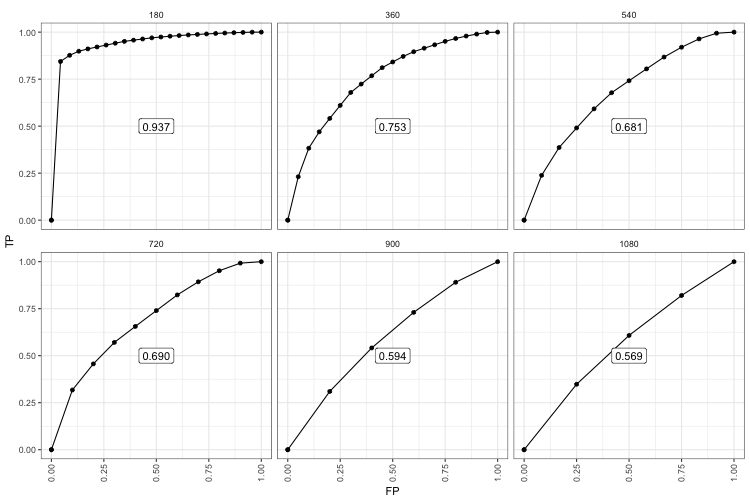
The difference is clearer in the later period. Most notably, only individuals that are in the risk set at each time point contribute data. So there are fewer data points. The decay in performance is clearer perhaps because among those who survived long enough the time-zero risk score is not as relevant. Once there are not events left, the ROC essentially flat-lined.
Conclusion
In conclusion, we examined two definitions of time-dependent ROC and their R implementation. The cumulative case/dynamic control ROC is likely more compatible with the notion of risk (cumulative incidence) prediction models. The incident case/dynamic control ROC may be of use for examining how long the time-zero marker remains relevant in predicting later events.
References
- Heagerty, Patrick J. and Zheng, Yingye, Survival Model Predictive Accuracy and ROC Curves, Biometrics, 61(1), pp. 92-105 (2005). doi:10.1111/j.0006-341X.2005.030814.x.
- Heagerty, P. J.; Lumley, T. and Pepe, M. S., Time-Dependent ROC Curves for Censored Survival Data and a Diagnostic Marker, Biometrics, 56(2), pp. 337-344 (2000). doi:10.1111/j.0006-341X.2000.00337.x.
- Edmonson, J. H.; Fleming, T. R.; Decker, D. G.; Malkasian, G. D.; Jorgensen, E. O.; Jefferies, J. A.; Webb, M. J. and Kvols, L. K., Different Chemotherapeutic Sensitivities and Host Factors Affecting Prognosis in Advanced Ovarian Carcinoma versus Minimal Residual Disease, Cancer Treat Rep, 63(2), pp. 241-247 (1979).