Even though the libraries for R from Python, or Python from R code execution existed since years and despite of a recent announcement of Ursa Labs foundation by Wes McKinney who is aiming to join forces with RStudio foundation, Hadley Wickham in particularly, (find more here) to improve data scientists workflow and unify libraries to be used not only in Python, but in any programming language used by data scientists, some data professionals are still very strict on the language to be used for ANN models limiting their dev. environment exclusively to Python.
As a continuation of my R vs. Python comparison, I decided to test performance of both languages in terms of time required to train a convolutional neural network based model for image recognition. As the starting point, I took the blog post by Dr. Shirin Glander on how easy it is to build a CNN model in R using Keras.
A few words about Keras. It is a Python library for artificial neural network ML models which provides high level fronted to various deep learning frameworks with Tensorflow being the default one.
Keras has many pros with the following among the others:
- Easy to build complex models just in few lines of code => perfect for dev. cycle to quickly experiment and check your ideas
- Code recycling: one can easily swap the backend framework (let’s say from CNTK to Tensorflow or vice versa) => DRY principle
- Seamless use of GPU => perfect for fast model tuning and experimenting
Since Keras is written in Python, it may be a natural choice for your dev. environment to use Python. And that was the case until about a year ago when RStudio founder J.J.Allaire announced release of the Keras library for R in May’17. I consider this to be a turning point for data scientists; now we can be more flexible with dev. environment and be able to deliver result more efficiently with opportunity to extend existing solutions we may have written in R.
It brings me to the point of this post.
My hypothesis is, when it comes to ANN ML model building with Keras, Python is not a must, and depending on your client’s request, or tech stack, R can be used without limitations and with similar efficiency.
Image Classification with Keras
In order to test my hypothesis, I am going to perform image classification using the fruit images data from kaggle and train a CNN model with four hidden layers: two 2D convolutional layers, one pooling layer and one dense layer. RMSProp is being used as the optimizer function.
Tech stack
Hardware:
CPU: Intel Core i7-7700HQ: 4 cores (8 threads), 2800 – 3800 (Boost) MHz core clock
GPU: Nvidia Geforce GTX 1050 Ti Mobile: 4Gb vRAM, 1493 – 1620 (Boost) MHz core clock
RAM: 16 Gb
Software:
OS: Linux Ubuntu 16.04
R: ver. 3.4.4
Python: ver. 3.6.3
Keras: ver. 2.2
Tensorflow: ver. 1.7.0
CUDA: ver. 9.0 (note that the current tensorflow version supports ver. 9.0 while the up-to-date version of cuda is 9.2)
cuDNN: ver. 7.0.5 (note that the current tensorflow version supports ver. 7.0 while the up-to-date version of cuDNN is 7.1)
Code
The R and Python code snippets used for CNN model building are present bellow. Thanks to fruitful collaboration between F. Chollet and J.J. Allaire, the logic and functions names in R are alike the Python ones.
R
## Courtesy: Dr. Shirin Glander. Code source: https://shirinsplayground.netlify.com/2018/06/keras_fruits/

library(keras)
start <- Sys.time()
fruit_list <- c("Kiwi", "Banana", "Plum", "Apricot", "Avocado", "Cocos", "Clementine", "Mandarine", "Orange",
                "Limes", "Lemon", "Peach", "Plum", "Raspberry", "Strawberry", "Pineapple", "Pomegranate")

# number of output classes (i.e. fruits)
output_n <- length(fruit_list)

# image size to scale down to (original images are 100 x 100 px)
img_width <- 20
img_height <- 20
target_size <- c(img_width, img_height)

# RGB = 3 channels
channels <- 3

# path to image folders
path <- "path/to/folder/with/data"
train_image_files_path <- file.path(path, "fruits-360", "Training")
valid_image_files_path <- file.path(path, "fruits-360", "Test")

# optional data augmentation
train_data_gen %>% image_data_generator(
  rescale = 1/255
)

# Validation data shouldn't be augmented! But it should also be scaled.
valid_data_gen <- image_data_generator(
  rescale = 1/255
)

# training images
train_image_array_gen <- flow_images_from_directory(train_image_files_path,
                                                    train_data_gen,
                                                    target_size = target_size,
                                                    class_mode = 'categorical',
                                                    classes = fruit_list,
                                                    seed = 42)

# validation images
valid_image_array_gen <- flow_images_from_directory(valid_image_files_path,
                                                    valid_data_gen,
                                                    target_size = target_size,
                                                    class_mode = 'categorical',
                                                    classes = fruit_list,
                                                    seed = 42)

### model definition
# number of training samples
train_samples <- train_image_array_gen$n
# number of validation samples
valid_samples <- valid_image_array_gen$n

# define batch size and number of epochs
batch_size <- 32
epochs <- 10

# initialise model
model <- keras_model_sequential()

# add layers
model %>%
  layer_conv_2d(filter = 32, kernel_size = c(3,3), padding = 'same', input_shape = c(img_width, img_height, channels)) %>%
  layer_activation('relu') %>%

  # Second hidden layer
  layer_conv_2d(filter = 16, kernel_size = c(3,3), padding = 'same') %>%
  layer_activation_leaky_relu(0.5) %>%
  layer_batch_normalization() %>%

  # Use max pooling
  layer_max_pooling_2d(pool_size = c(2,2)) %>%
  layer_dropout(0.25) %>%

  # Flatten max filtered output into feature vector
  # and feed into dense layer
  layer_flatten() %>%
  layer_dense(100) %>%
  layer_activation('relu') %>%
  layer_dropout(0.5) %>%

  # Outputs from dense layer are projected onto output layer
  layer_dense(output_n) %>%
  layer_activation('softmax')

# compile
model %>% compile(
  loss = 'categorical_crossentropy',
  optimizer = optimizer_rmsprop(lr = 0.0001, decay = 1e-6),
  metrics = 'accuracy'
)
# fit
hist <- fit_generator(
  # training data
  train_image_array_gen,

  # epochs
  steps_per_epoch = as.integer(train_samples / batch_size),
  epochs = epochs,

  # validation data
  validation_data = valid_image_array_gen,
  validation_steps = as.integer(valid_samples / batch_size),

  # print progress
  verbose = 2,
  callbacks = list(
    # save best model after every epoch
    callback_model_checkpoint(file.path(path, "fruits_checkpoints.h5"), save_best_only = TRUE),
    # only needed for visualising with TensorBoard
    callback_tensorboard(log_dir = file.path(path, "fruits_logs"))
  )
)

df_out <- hist$metrics %>%
  {data.frame(acc = .$acc[epochs], val_acc = .$val_acc[epochs], elapsed_time = as.integer(Sys.time()) - as.integer(start))}
Python
## Author: D. Kisler  - adoptation of R code from https://shirinsplayground.netlify.com/2018/06/keras_fruits/

from keras.preprocessing.image import ImageDataGenerator
from keras.models import Sequential
from keras.layers import (Conv2D,
                          Dense,
                          LeakyReLU,
                          BatchNormalization,
                          MaxPooling2D,
                          Dropout,
                          Flatten)
from keras.optimizers import RMSprop
from keras.callbacks import ModelCheckpoint, TensorBoard
import PIL.Image
from datetime import datetime as dt

start = dt.now()

# fruits categories
fruit_list = ["Kiwi", "Banana", "Plum", "Apricot", "Avocado", "Cocos", "Clementine", "Mandarine", "Orange",
                "Limes", "Lemon", "Peach", "Plum", "Raspberry", "Strawberry", "Pineapple", "Pomegranate"]
# number of output classes (i.e. fruits)
output_n = len(fruit_list)
# image size to scale down to (original images are 100 x 100 px)
img_width = 20
img_height = 20
target_size = (img_width, img_height)
# image RGB channels number
channels = 3
# path to image folders
path = "path/to/folder/with/data"
train_image_files_path = path + "fruits-360/Training"
valid_image_files_path = path + "fruits-360/Test"

## input data augmentation/modification
# training images
train_data_gen = ImageDataGenerator(
  rescale = 1./255
)
# validation images
valid_data_gen = ImageDataGenerator(
  rescale = 1./255
)

## getting data
# training images
train_image_array_gen = train_data_gen.flow_from_directory(train_image_files_path,
                                                           target_size = target_size,
                                                           classes = fruit_list,
                                                           class_mode = 'categorical',
                                                           seed = 42)

# validation images
valid_image_array_gen = valid_data_gen.flow_from_directory(valid_image_files_path,
                                                           target_size = target_size,
                                                           classes = fruit_list,
                                                           class_mode = 'categorical',
                                                           seed = 42)

## model definition
# number of training samples
train_samples = train_image_array_gen.n
# number of validation samples
valid_samples = valid_image_array_gen.n
# define batch size and number of epochs
batch_size = 32
epochs = 10

# initialise model
model = Sequential()

# add layers
# input layer
model.add(Conv2D(filters = 32, kernel_size = (3,3), padding = 'same', input_shape = (img_width, img_height, channels), activation = 'relu'))
# hiddel conv layer
model.add(Conv2D(filters = 16, kernel_size = (3,3), padding = 'same'))
model.add(LeakyReLU(.5))
model.add(BatchNormalization())
# using max pooling
model.add(MaxPooling2D(pool_size = (2,2)))
# randomly switch off 25% of the nodes per epoch step to avoid overfitting
model.add(Dropout(.25))
# flatten max filtered output into feature vector
model.add(Flatten())
# output features onto a dense layer
model.add(Dense(units = 100, activation = 'relu'))
# randomly switch off 25% of the nodes per epoch step to avoid overfitting
model.add(Dropout(.5))
# output layer with the number of units equal to the number of categories
model.add(Dense(units = output_n, activation = 'softmax'))

# compile the model
model.compile(loss = 'categorical_crossentropy',
              metrics = ['accuracy'],
              optimizer = RMSprop(lr = 1e-4, decay = 1e-6))

# train the model
hist = model.fit_generator(
  # training data
  train_image_array_gen,

  # epochs
  steps_per_epoch = train_samples // batch_size,
  epochs = epochs,

  # validation data
  validation_data = valid_image_array_gen,
  validation_steps = valid_samples // batch_size,

  # print progress
  verbose = 2,
  callbacks = [
    # save best model after every epoch
    ModelCheckpoint("fruits_checkpoints.h5", save_best_only = True),
    # only needed for visualising with TensorBoard
    TensorBoard(log_dir = "fruits_logs")
  ]
)

df_out = {'acc': hist.history['acc'][epochs - 1], 'val_acc': hist.history['val_acc'][epochs - 1], 'elapsed_time': (dt.now() - start).seconds}
Experiment
The models above were trained 10 times with R and Pythons on GPU and CPU, the elapsed time and the final accuracy after 10 epochs were measured. The results of the measurements are presented on the plots below (click the plot to be redirected to plotly interactive plots).
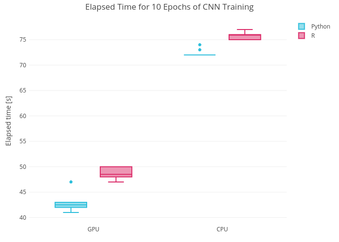
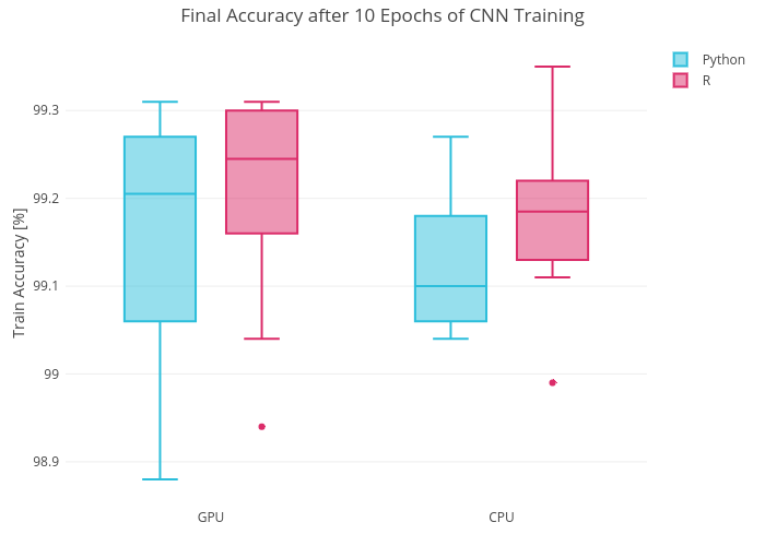
From the plots above, one can see that:
- the accuracy of your model doesn’t depend on the language you use to build and train it (the plot shows only train accuracy, but the model doesn’t have high variance and the bias accuracy is around 99% as well).
- even though 10 measurements may be not convincing, but Python would reduce (by up to 15%) the time required to train your CNN model. This is somewhat expected because R uses Python under the hood when executes Keras functions.
Let’s perform unpaired t-test assuming that all our observations are normally distributed.
library(dplyr)
library(data.table)
# fetch the data used to plot graphs
d <- fread('keras_elapsed_time_rvspy.csv')

# unpaired t test:
# t_score = (mean1 - mean2)/sqrt(stdev1^2/n1+stdev2^2/n2)

d %>%
    group_by(lang, eng) %>%
    summarise(el_mean = mean(elapsed_time),
              el_std = sd(elapsed_time),
              n = n()) %>% data.frame() %>%
    group_by(eng) %>%
    summarise(t_score = round(diff(el_mean)/sqrt(sum(el_std^2/n)), 2))
| eng | t_score |
|---|---|
| cpu | 11.38 |
| gpu | 9.64 |
T-score reflects a significant difference between the time required to train a CNN model in R compared to Python as we saw on the plot above.
Summary
Building and training CNN model in R using Keras is as “easy” as in Python with the same coding logic and functions naming convention. Final accuracy of your Keras model will depend on the neural net architecture, hyperparameters tuning, training duration, train/test data amount etc., but not on the programming language you would use for your DS project. Training a CNN Keras model in Python may be up to 15% faster compared to R
P.S.
If you would like to know more about Keras and to be able to build models with this awesome library, I recommend you these books:
- Deep Learning with Python by F. Chollet (one of the Keras creators)
- Deep Learning with R by F. Chollet and J.J. Allaire
As well as this Udemy course to start your journey with Keras.
Thanks a lot for your attention! I hope this post would be helpful for an aspiring data scientist to gain an understanding of use cases for different technologies and to avoid being biased when it comes to the selection of the tools for DS projects accomplishment.
It is nonsensical to test language A against language B using a package developed for language A. R supports tensorflow directly so use tensorflow or MSNetR or several other CNN-capable packages specifically for R. Comparisons like this one, however, are simply silly.