We are continuing on with our NYC bus breakdown problem. When we left off, we had constructed a rule-based Cubist regression model with our expanded pool of predictors; but we were still only managing to explain 37% of the data's variance with our model. Given how 'dirty' the target variable 'time_delayed' is (because it is human reported and of dubious precision), we decided that perhaps we should rephrase the question in order to get a more sensible answer. When a bus breakdown is called into operations, perhaps the question to ask is: “Will this delay exceed twenty minutes?”
Classification – more than 20 minutes?
We could choose some other time, but for simplicity, twenty minutes is probably the breaking point of human patience – be they, passengers or providers. This division also breaks the dataset approximately in half, so we don't have to deal with imbalance. As a side note, I have also run the problem for a thirty minute or more delay, breaking the data into ¾ and ¼; and the solution only improves.
We begin by setting up the data that we need, and the caret control objects:
in_csv <- "../output/intermediate/ii_times.csv"
ii_times <- read_csv(in_csv) %>%
  filter(reported_before_resolved == 1) %>%
  select(-reported_before_resolved) %>%
  mutate(
    time_delayed = cut(time_delayed, breaks = c(0, 22, 10000), labels = FALSE)
  ) %>%
  mutate(time_delayed = factor(time_delayed, labels = c("t0.22","t22.")))
halfFold <- createFolds(ii_times$Busbreakdown_ID, k = 5, list=TRUE)
ii_small <- ii_times[halfFold[[2]],]
ii_test <-ii_times[halfFold[[3]],]
ii_train <- ii_times %>%
  anti_join(ii_test, by = "Busbreakdown_ID")
rctrl_manual <- trainControl(method = "none", returnResamp = "all", classProbs = TRUE, summaryFunction = twoClassSummary)
rctrl_repcv <- trainControl(method = "repeatedcv", number = 2, repeats = 5, returnResamp = "all", classProbs = TRUE, summaryFunction = twoClassSummary)
Then we can use cross-fold validation on a reduced data set to quickly get a sense of which parameters we should use. Note that we deliberately choose 'rules', not 'tree' here, because we want a human-readable set of if/then conditions. Unfortunately, we will end up using 15 trials, which means our rule set is large. I have commented its output here, but it can be read this way, or with 'summary(model)'.
#---cubist
c50_grd<-expand.grid(
  .winnow = FALSE,
  .trials=c(15,30,50),
  .model="rules"
)
set.seed(849)
c50_cv <- train(time_delayed ~ . -Busbreakdown_ID,
  data = ii_small,
  method = "C5.0",
  metric="ROC",
  na.action = na.pass,
  trControl = rctrl_repcv,
  tuneGrid = c50_grd
  )
c50_cv
## C5.0
##
## 40665 samples
##    46 predictor
##     2 classes: 't0.22', 't22.'
##
## No pre-processing
## Resampling: Cross-Validated (2 fold, repeated 5 times)
## Summary of sample sizes: 20332, 20333, 20332, 20333, 20332, 20333, ...
## Resampling results across tuning parameters:
##
##   trials  ROC        Sens       Spec
##   15      0.8261069  0.8028816  0.6830990
##   30      0.8258429  0.8030490  0.6855583
##   50      0.8258429  0.8030490  0.6855583
##
## Tuning parameter 'model' was held constant at a value of rules
##
## Tuning parameter 'winnow' was held constant at a value of FALSE
## ROC was used to select the optimal model using the largest value.
## The final values used for the model were trials = 15, model = rules
##  and winnow = FALSE.
#writeLines(c50_cv$finalModel$rules)
#We can output the rule set as a block of text like this, but we have suppressed this output because with 50 trials, it is a very, very long list.
The system is relatively insensitive to the number of trials, so we can use 15. We run on our training and test sets to derive our true test ROC, and have a look at how our predicted probabilities correlate with the predictors, compared to the actual values.
c50_grd<-expand.grid(
  .winnow = FALSE,
  .trials=15,
  .model="rules"
)
c50_man <- train(time_delayed ~ . -Busbreakdown_ID,
  data = ii_train,
  method = "C5.0",
  metric="ROC",
  na.action = na.pass,
  trControl = rctrl_manual,
  tuneGrid = c50_grd
)
predictions <- predict(c50_man, newdata = ii_test, type = "prob")
ii_withpred <- ii_test %>%
  cbind(predictions %>% tbl_df())
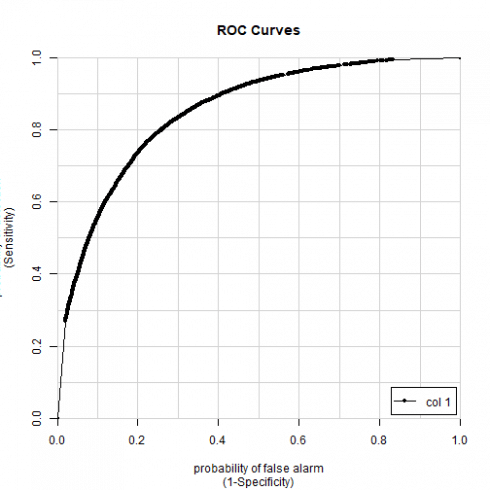
colAUC(ii_withpred[["t0.22"]], (ii_withpred[["time_delayed"]] =="t0.22") * 1L, plotROC=TRUE)

##              [,1]
## 0 vs. 1 0.8486122
#cubist: 0.847
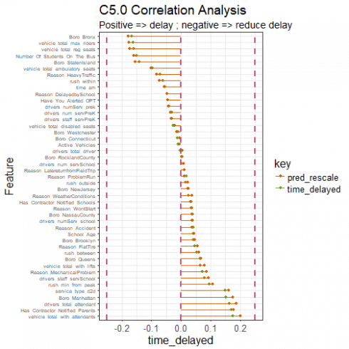
corrr_analysis <- ii_withpred %>%
  select(-Busbreakdown_ID, -t0.22, -t22.) %>%
  mutate(
    time_delayed = (time_delayed == "t22.")*1L
  ) %>%
  correlate() %>%
  focus(time_delayed) %>%
  rename(feature = rowname) %>%
  arrange(desc(abs(time_delayed))) %>%
  mutate(feature = as_factor(feature))
corrr_analysis %>% print(n=61)
## # A tibble: 45 x 2
##    feature                         time_delayed
##    <fct>                                  <dbl>
##  1 vehicle_total_with_attendants        0.176
##  2 Has_Contractor_Notified_Parents      0.171
##  3 Boro_Bronx                          -0.165
##  4 drivers_total_attendant              0.163
##  5 vehicle_total_max_riders            -0.162
##  6 vehicle_total_reg_seats             -0.160
##  7 Boro_Manhattan                       0.151
##  8 service_type_d2d                     0.149
##  9 Number_Of_Students_On_The_Bus       -0.149
## 10 Boro_StatenIsland                   -0.140
## 11 vehicle_total_ambulatory_seats      -0.0972
## 12 rush_min_from_peak                   0.0954
## 13 drivers_staff_servSchool             0.0792
## 14 Reason_MechanicalProblem             0.0729
## 15 Reason_HeavyTraffic                 -0.0698
## 16 Boro_Queens                          0.0667
## 17 vehicle_total_with_lifts             0.0654
## 18 rush_within                         -0.0612
## 19 time_am                             -0.0545
## 20 rush_between                         0.0538
## 21 Reason_DelayedbySchool              -0.0471
## 22 Reason_FlatTire                      0.0461
## 23 Have_You_Alerted_OPT                -0.0457
## 24 Reason_Accident                      0.0427
## 25 Boro_Brooklyn                        0.0421
## 26 School_Age                           0.0416
## 27 drivers_numServ_prek                -0.0394
## 28 Boro_NassauCounty                    0.0389
## 29 drivers_numServ_school               0.0374
## 30 Reason_WontStart                     0.0371
## 31 Has_Contractor_Notified_Schools      0.0346
## 32 drivers_num_servPreK                -0.0315
## 33 drivers_staff_servPreK              -0.0305
## 34 Reason_WeatherConditions             0.0264
## 35 vehicle_total_disabled_seats        -0.0252
## 36 Boro_NewJersey                       0.0236
## 37 Reason_ProblemRun                    0.0193
## 38 rush_outside                         0.0164
## 39 Boro_Connecticut                    -0.0110
## 40 Active_Vehicles                     -0.0108
## 41 Boro_Westchester                    -0.0103
## 42 Reason_LatereturnfromFieldTrip       0.0102
## 43 Boro_RocklandCounty                  0.00316
## 44 drivers_num_servSchool               0.00243
## 45 drivers_total_driver                -0.00199
corrr_pred <- ii_withpred %>%
  select(-Busbreakdown_ID, -time_delayed, -t0.22) %>%
  correlate() %>%
  focus(t22.) %>%
  rename(feature = rowname) %>%
  arrange(desc(abs(t22.))) %>%
  mutate(feature = as_factor(feature))
corrr_full <- corrr_analysis %>%
  left_join(corrr_pred, by = "feature") %>%
  mutate(
    #pred_rescale = t22.,
    pred_rescale = t22. * median(abs(time_delayed)) / median(abs(t22.)),
    t22. = NULL
  ) %>%
  gather(key = key, value = time_delayed, -feature)
pal <- brewer.pal(8, "Dark2")
corrr_full %>%
  ggplot(aes(x = time_delayed, y = fct_reorder(feature, desc(time_delayed)), color = key)) +
  geom_point() +
  scale_color_manual(values = c(pal[2],pal[5])) +
  # Positive Correlations - Contribute to churn
  geom_segment(aes(xend = 0, yend = feature, color = key),
    data = corrr_full %>% filter(time_delayed > 0)) +
  # Negative Correlations - Prevent churn
  geom_segment(aes(xend = 0, yend = feature, color = key),
    data = corrr_full %>% filter(time_delayed < 0)) +
  # Vertical lines
  geom_vline(xintercept = 0, color = plasma(3)[[2]], size = 1, linetype = 2) +
  geom_vline(xintercept = -0.25, color = plasma(3)[[2]], size = 1, linetype = 2) +
  geom_vline(xintercept = 0.25, color = plasma(3)[[2]], size = 1, linetype = 2) +
  # Aesthetics
  theme_bw() +
  labs(title = "C5.0 Correlation Analysis",
    subtitle = paste("Positive => delay",
      "; negative => reduce delay"),
    y = "Feature") +
  theme(text=element_text(family="Arial", size=16), axis.text.y = element_text(size=7))
Our ROC is 0.848, which we cannot complain about. Our predictions correlate with our predictors as expected. With a fairly limited set of predictors, and despite our very dirty target variable, we can be reasonably certain whether a delay will be greater or less than twenty minutes. But, of course, we should keep in mind that the equivalent regression is rather bad. We have had to choose our poison, and have made do.
I am leaving this data problem here. There is more than I could do to add predictors. One thing that I wanted to do at the outset of this problem was finding the geospatial data for the routes themselves, and see if I could add predictors based on neighborhood council fees, or house prices, or crime statistics, or the number of dogs / birds / trees, or whatever else seemed fun. But I have come far enough with this (for now) and will be moving on to something different. If you would like any of the ‘cleaner’ data, let me know and I’ll see what I can do.

