We use normality tests when we want to understand whether a given sample set of continuous (variable) data could have come from the Gaussian distribution (also called the normal distribution). Normality tests are a pre-requisite for some inferential statistics, especially the generation of confidence intervals and hypothesis tests such as 1 and 2 sample t-tests. The normality assumption is also important when we’re performing ANOVA, to compare multiple samples of data with one another to determine if they come from the same population. Normality tests are a form of hypothesis test, which is used to make an inference about the population from which we have collected a sample of data. There are a number of normality tests available for R. All these tests fundamentally assess the below hypotheses. The first of these is called a null hypothesis – which states that there is no difference between this data set and the normal distribution.
- H0: No observable difference between data and normal distribution
- Ha: Clear observable difference between data and normal distribution
The alternative hypothesis, which is the second statement, is the logical opposite of the null hypothesis in each hypothesis test. Based on the test results, we can take decisions about what further kinds of testing we can use on the data. For instance, for two samples of data to be able to compared using 2-sample t-tests, they should both come from normal distributions, and should have similar variances.
Normality tests are not present in the base packages of R, but are present in the nortest package. To install nortest, simply type the following command in your R console window.
install.packages("nortest")
Once the package is installed, you can run one of the many different types of normality tests when you do data analysis. Let’s look at the most common normality test, the Anderson-Darling normality test, in this tutorial. We’ll use two different samples of data in each case, and compare the results for each sample.
Anderson-Darling Normality Test
The Anderson-Darling test (AD test, for short) is one of the most commonly used normality tests, and can be executed using the ad.test() command present within the nortest package.
#Invoking the "nortest" package into the active R session
library(nortest)

#Generating a sample of 100 random numbers from a Gaussian / normal distribution
x <- rnorm(100,10,1)

#Generating a sample of 100 numbers from a non-normal data set
y <- rweibull(100,1,5)
Interpreting Normality Test Results
When the ad.test() command is run, the results include test statistics and p-values. The results for the above Anderson-Darling tests are shown below:
ad.test(x)
ad.test(y)
	Anderson-Darling normality test
data:  x
A = 0.1595, p-value = 0.9482

	Anderson-Darling normality test
data:  y
A = 4.9867, p-value = 2.024e-12
As you can see clearly above, the results from the test are different for the two different samples of data. One of these samples, x, came from a normal distribution, and the p-value of the normality test done on that sample was 0.9482. This means, that if we were to assume the default (null) hypothesis to be true, there is a 94.82% chance that you would see a result as extreme or more extreme from the same distribution where this sample was collected. Naturally, this means that there is a very high likelihood of this data set having come from a normal distribution.
Let us now look at the result from the second data set’s test. The p-value of the normality test done on this data set (y, which was not generated from a normal distribution), is very low, indicating that if the null hypothesis (that the data came from the normal distribution) were to be true, there would be a very small chance of seeing the same kind of sample from such a distribution. Therefore, the Anderson-Darling normality test is able to tell the difference between a sample of data from the normal distribution, and another sample, which is not from the normal distribution, based on the test-statistic.
Quantile Plots in R
Visually, we can study the impact of the parent distribution of any sample data, by using normal quantile plots.
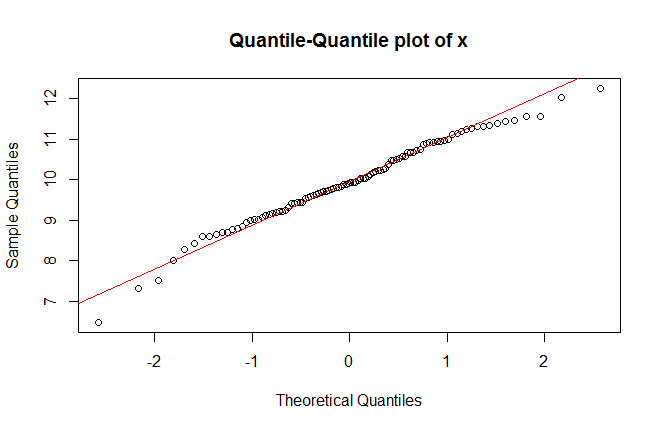
Normal Quantile-Quantile plot for sample ‘x’
qqnorm(x)
qqline(x, col = "red")
Normal Quantile-Quantile plot for sample ‘y’
qqnorm(y)
qqline(y, col = "red")
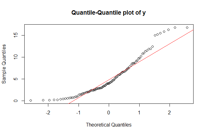
Normal Q-Q plots help us understand whether the quantiles in a data set are similar to that which you can expect in normally distributed data. When you see a Normal Q-Q plot where the points in the sample are lined up along the line generated by the qqline() command, you’re seeing a sample that could very well be from a normal distribution. In general, when you see the points arranged on a curve, and points far away from the line on the Q-Q plot, it indicates a tendency towards non-normality. Observe how in the Normal Q-Q plot for sample ‘y’, the points are lined up along a curve, and don’t coincide very well with the line generated by qqline().
Non-normal Data
In the example data sets shown here, one of the samples, y, comes from a non-normal data set. It is common enough to find continuous data from processes that could be described using log-normal, logistic, Weibull and other distributions. There are also methods of transforming data using transformation methods, like the Box-Cox transformation, or the Johnson transformation, which help convert data sets from non-normal to normal data sets. When conducting hypothesis tests using non-normal data sets, we can use methods like the Wilcoxon, Mann-Whitney and Moods-Median tests to compare ranked means or medians, rather than means, as estimators for non-normal data.
Conclusion and remarks
The A-D test is susceptible to extreme values, and may not give good results for very large data sets. In such situations, it is advisable to use other normality tests such as the Shapiro-Wilk test. As a good practice, consider constructing quantile plots, which can also help understand the distribution of your data set. Normality tests can be useful prior to activities such as hypothesis testing for means (1-sample and 2-sample t-tests). The practical use of such tests is in performance testing of engineering systems, AB testing of websites, and in engineering, medical and biological laboratories. The test can also be used in process excellence teams as a precursor to process capability analysis.