About one in seven U.S. adults has diabetes now, according to the Centers for Disease Control and Prevention. But by 2050, that rate could skyrocket to as many as one in three. With this in mind, this is what we are going to do today: Learning how to use Machine Learning to help us predict Diabetes. Let’s get started!
The Data
The diabetes data set was originated from UCI Machine Learning Repository and can be downloaded from here
import pandas as pd
import numpy as np
import matplotlib.pyplot as plt
%matplotlib inline
diabetes = pd.read_csv('diabetes.csv')
print(diabetes.columns)
Index([‘Pregnancies’, ‘Glucose’, ‘BloodPressure’, ‘SkinThickness’, ‘Insulin’, ‘BMI’, ‘DiabetesPedigreeFunction’, ‘Age’, ‘Outcome’], dtype=’object’)
diabetes.head()
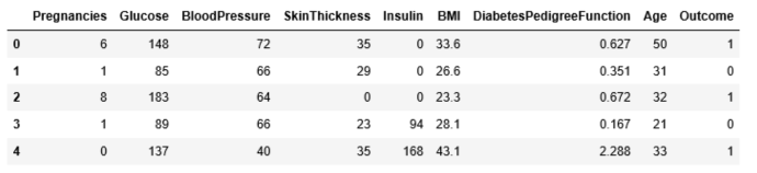
The diabetes data set consists of 768 data points, with 9 features each:
print("dimension of diabetes data: {}".format(diabetes.shape))
dimension of diabetes data: (768, 9)
“Outcome” is the feature we are going to predict, 0 means No diabetes, 1 means diabetes. Of these 768 data points, 500 are labeled as 0 and 268 as 1:
print(diabetes.groupby('Outcome').size())
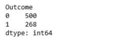
import seaborn as sns
sns.countplot(diabetes['Outcome'],label="Count")
Gives this plot:
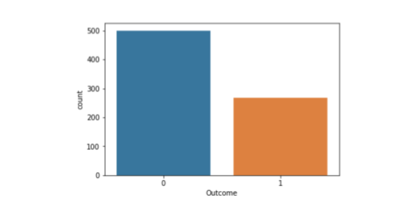
diabetes.info()
k-Nearest Neighbors
The k-NN algorithm is arguably the simplest machine learning algorithm. Building the model consists only of storing the training data set. To make a prediction for a new data point, the algorithm finds the closest data points in the training data set — its “nearest neighbors.”
First, Let’s investigate whether we can confirm the connection between model complexity and accuracy:
from sklearn.model_selection import train_test_split
X_train, X_test, y_train, y_test = train_test_split(diabetes.loc[:, diabetes.columns != 'Outcome'], diabetes['Outcome'], stratify=diabetes['Outcome'], random_state=66)
from sklearn.neighbors import KNeighborsClassifier
training_accuracy = []
test_accuracy = []
# try n_neighbors from 1 to 10
neighbors_settings = range(1, 11)
for n_neighbors in neighbors_settings:
    # build the model
    knn = KNeighborsClassifier(n_neighbors=n_neighbors)
    knn.fit(X_train, y_train)
    # record training set accuracy
    training_accuracy.append(knn.score(X_train, y_train))
    # record test set accuracy
    test_accuracy.append(knn.score(X_test, y_test))
plt.plot(neighbors_settings, training_accuracy, label="training accuracy")
plt.plot(neighbors_settings, test_accuracy, label="test accuracy")
plt.ylabel("Accuracy")
plt.xlabel("n_neighbors")
plt.legend()
plt.savefig('knn_compare_model')
Gives this plot:
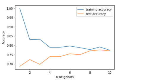
The above plot shows the training and test set accuracy on the y-axis against the setting of n_neighbors on the x-axis. Considering if we choose one single nearest neighbor, the prediction on the training set is perfect. But when more neighbors are considered, the training accuracy drops, indicating that using the single nearest neighbor leads to a model that is too complex. The best performance is somewhere around 9 neighbors.
The plot suggests that we should choose n_neighbors=9. Here we are:
knn = KNeighborsClassifier(n_neighbors=9)
knn.fit(X_train, y_train)
print('Accuracy of K-NN classifier on training set: {:.2f}'.format(knn.score(X_train, y_train)))
print('Accuracy of K-NN classifier on test set: {:.2f}'.format(knn.score(X_test, y_test)))
Accuracy of K-NN classifier on training set: 0.79
Accuracy of K-NN classifier on test set: 0.78
Logistic regression
Logistic Regression is one of the most common classification algorithms.
from sklearn.linear_model import LogisticRegression
logreg = LogisticRegression().fit(X_train, y_train)
print("Training set score: {:.3f}".format(logreg.score(X_train, y_train)))
print("Test set score: {:.3f}".format(logreg.score(X_test, y_test)))
Training set accuracy: 0.781
Test set accuracy: 0.771
The default value of C=1 provides with 78% accuracy on the training and 77% accuracy on the test set.
logreg001 = LogisticRegression(C=0.01).fit(X_train, y_train)
print("Training set accuracy: {:.3f}".format(logreg001.score(X_train, y_train)))
print("Test set accuracy: {:.3f}".format(logreg001.score(X_test, y_test)))
Training set accuracy: 0.700
Test set accuracy: 0.703
Using C=0.01 results in lower accuracy on both the training and the test sets.
logreg100 = LogisticRegression(C=100).fit(X_train, y_train)
print("Training set accuracy: {:.3f}".format(logreg100.score(X_train, y_train)))
print("Test set accuracy: {:.3f}".format(logreg100.score(X_test, y_test)))
Training set accuracy: 0.785
Test set accuracy: 0.766
Using C=100 results in a little bit higher accuracy on the training set and little bit lower accuracy on the test set, confirming that less regularization and a more complex model may not generalize better than default setting.
Therefore, we should choose default value C=1.
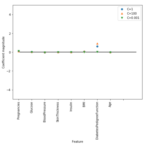
Let’s visualize the coefficients learned by the models with the three different settings of the regularization parameter C.
Stronger regularization (C=0.001) pushes coefficients more and more toward zero. Inspecting the plot more closely, we can also see that feature “DiabetesPedigreeFunction”, for C=100, C=1 and C=0.001, the coefficient is positive. This indicates that high “DiabetesPedigreeFunction” feature is related to a sample being “diabetes”, regardless which model we look at.
diabetes_features = [x for i,x in enumerate(diabetes.columns) if i!=8]
plt.figure(figsize=(8,6))
plt.plot(logreg.coef_.T, 'o', label="C=1")
plt.plot(logreg100.coef_.T, '^', label="C=100")
plt.plot(logreg001.coef_.T, 'v', label="C=0.001")
plt.xticks(range(diabetes.shape[1]), diabetes_features, rotation=90)
plt.hlines(0, 0, diabetes.shape[1])
plt.ylim(-5, 5)
plt.xlabel("Feature")
plt.ylabel("Coefficient magnitude")
plt.legend()
plt.savefig('log_coef')
Gives this plot:
Decision Tree
from sklearn.tree import DecisionTreeClassifier
tree = DecisionTreeClassifier(random_state=0)
tree.fit(X_train, y_train)
print("Accuracy on training set: {:.3f}".format(tree.score(X_train, y_train)))
print("Accuracy on test set: {:.3f}".format(tree.score(X_test, y_test)))
Accuracy on training set: 1.000
Accuracy on test set: 0.714
The accuracy on the training set is 100%, while the test set accuracy is much worse. This is an indicative that the tree is overfitting and not generalizing well to new data. Therefore, we need to apply pre-pruning to the tree.
We set max_depth=3, limiting the depth of the tree decreases overfitting. This leads to a lower accuracy on the training set, but an improvement on the test set.
tree = DecisionTreeClassifier(max_depth=3, random_state=0)
tree.fit(X_train, y_train)
print("Accuracy on training set: {:.3f}".format(tree.score(X_train, y_train)))
print("Accuracy on test set: {:.3f}".format(tree.score(X_test, y_test)))
Accuracy on training set: 0.773
Accuracy on test set: 0.740
Feature Importance in Decision Trees
Feature importance rates how important each feature is for the decision a tree makes. It is a number between 0 and 1 for each feature, where 0 means “not used at all” and 1 means “perfectly predicts the target”. The feature importances always sum to 1:
print("Feature importances:\n{}".format(tree.feature_importances_))
Feature importances: [ 0.04554275 0.6830362 0. 0. 0. 0.27142106 0. 0. ]
Then we can visualize the feature importances:
def plot_feature_importances_diabetes(model):
    plt.figure(figsize=(8,6))
    n_features = 8
    plt.barh(range(n_features), model.feature_importances_, align='center')
    plt.yticks(np.arange(n_features), diabetes_features)
    plt.xlabel("Feature importance")
    plt.ylabel("Feature")
    plt.ylim(-1, n_features)
plot_feature_importances_diabetes(tree)
plt.savefig('feature_importance')
Gives this plot:
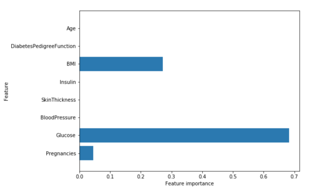
Feature “Glucose” is by far the most important feature.
Random Forest
Let’s apply a random forest consisting of 100 trees on the diabetes data set:
from sklearn.ensemble import RandomForestClassifier
rf = RandomForestClassifier(n_estimators=100, random_state=0)
rf.fit(X_train, y_train)
print("Accuracy on training set: {:.3f}".format(rf.score(X_train, y_train)))
print("Accuracy on test set: {:.3f}".format(rf.score(X_test, y_test)))
Accuracy on training set: 1.000
Accuracy on test set: 0.786
The random forest gives us an accuracy of 78.6%, better than the logistic regression model or a single decision tree, without tuning any parameters. However, we can adjust the max_features setting, to see whether the result can be improved.
rf1 = RandomForestClassifier(max_depth=3, n_estimators=100, random_state=0)
rf1.fit(X_train, y_train)
print("Accuracy on training set: {:.3f}".format(rf1.score(X_train, y_train)))
print("Accuracy on test set: {:.3f}".format(rf1.score(X_test, y_test)))
Accuracy on training set: 0.800
Accuracy on test set: 0.755
It did not, this indicates that the default parameters of the random forest work well.
Feature importance in Random Forest
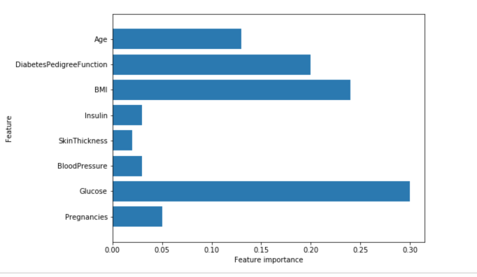
plot_feature_importances_diabetes(rf)
Gives this plot:
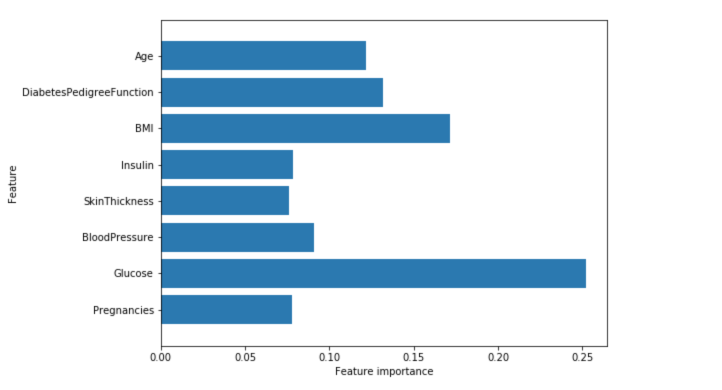
Similarly to the single decision tree, the random forest also gives a lot of importance to the “Glucose” feature, but it also chooses “BMI” to be the 2nd most informative feature overall. The randomness in building the random forest forces the algorithm to consider many possible explanations, the result being that the random forest captures a much broader picture of the data than a single tree.
Gradient Boosting
from sklearn.ensemble import GradientBoostingClassifier
gb = GradientBoostingClassifier(random_state=0)
gb.fit(X_train, y_train)
print("Accuracy on training set: {:.3f}".format(gb.score(X_train, y_train)))
print("Accuracy on test set: {:.3f}".format(gb.score(X_test, y_test)))
Accuracy on training set: 0.917
Accuracy on test set: 0.792
We are likely to be overfitting. To reduce overfitting, we could either apply stronger pre-pruning by limiting the maximum depth or lower the learning rate:
gb1 = GradientBoostingClassifier(random_state=0, max_depth=1)
gb1.fit(X_train, y_train)
print("Accuracy on training set: {:.3f}".format(gb1.score(X_train, y_train)))
print("Accuracy on test set: {:.3f}".format(gb1.score(X_test, y_test)))
Accuracy on training set: 0.804
Accuracy on test set: 0.781
gb2 = GradientBoostingClassifier(random_state=0, learning_rate=0.01)
gb2.fit(X_train, y_train)
print("Accuracy on training set: {:.3f}".format(gb2.score(X_train, y_train)))
print("Accuracy on test set: {:.3f}".format(gb2.score(X_test, y_test)))
Accuracy on training set: 0.802
Accuracy on test set: 0.776
Both methods of decreasing the model complexity reduced the training set accuracy, as expected. However, in this case, none of these methods increased the generalization performance of the test set.
We can visualize the feature importances to get more insight into our model even though we are not really happy with the model:
plot_feature_importances_diabetes(gb1)
Gives this plot:
We can see that the feature importances of the gradient boosted trees are somewhat similar to the feature importances of the random forests, it gives weight to all of the features in this case.
Support Vector Machine
from sklearn.svm import SVC
svc = SVC()
svc.fit(X_train, y_train)
print("Accuracy on training set: {:.2f}".format(svc.score(X_train, y_train)))
print("Accuracy on test set: {:.2f}".format(svc.score(X_test, y_test)))
Accuracy on training set: 1.00
Accuracy on test set: 0.65
The model overfits quite substantially, with a perfect score on the training set and only 65% accuracy on the test set.
SVM requires all the features to vary on a similar scale. We will need to re-scale our data that all the features are approximately on the same scale:
from sklearn.preprocessing import MinMaxScaler
scaler = MinMaxScaler()
X_train_scaled = scaler.fit_transform(X_train)
X_test_scaled = scaler.fit_transform(X_test)
svc = SVC()
svc.fit(X_train_scaled, y_train)
print("Accuracy on training set: {:.2f}".format(svc.score(X_train_scaled, y_train)))
print("Accuracy on test set: {:.2f}".format(svc.score(X_test_scaled, y_test)))
Accuracy on training set: 0.77
Accuracy on test set: 0.77
Scaling the data made a huge difference! Now we are actually underfitting, where training and test set performance are quite similar but less close to 100% accuracy. From here, we can try increasing either C or gamma to fit a more complex model.
svc = SVC(C=1000)
svc.fit(X_train_scaled, y_train)
print("Accuracy on training set: {:.3f}".format(
    svc.score(X_train_scaled, y_train)))
print("Accuracy on test set: {:.3f}".format(svc.score(X_test_scaled, y_test)))
Accuracy on training set: 0.790
Accuracy on test set: 0.797
Here, increasing C allows us to improve the model, resulting in 79.7% test set accuracy.
Deep Learning
from sklearn.neural_network import MLPClassifier
mlp = MLPClassifier(random_state=42)
mlp.fit(X_train, y_train)
print("Accuracy on training set: {:.2f}".format(mlp.score(X_train, y_train)))
print("Accuracy on test set: {:.2f}".format(mlp.score(X_test, y_test)))
Accuracy on training set: 0.71
Accuracy on test set: 0.67
The accuracy of the Multilayer perceptrons (MLP) is not as good as the other models at all, this is likely due to scaling of the data. deep learning algorithms also expect all input features to vary in a similar way, and ideally to have a mean of 0, and a variance of 1. We must re-scale our data so that it fulfills these requirements.
from sklearn.preprocessing import StandardScaler
scaler = StandardScaler()
X_train_scaled = scaler.fit_transform(X_train)
X_test_scaled = scaler.fit_transform(X_test)
mlp = MLPClassifier(random_state=0)
mlp.fit(X_train_scaled, y_train)
print("Accuracy on training set: {:.3f}".format(
    mlp.score(X_train_scaled, y_train)))
print("Accuracy on test set: {:.3f}".format(mlp.score(X_test_scaled, y_test)))
Accuracy on training set: 0.823
Accuracy on test set: 0.802
Let’s increase the number of iterations:
mlp = MLPClassifier(max_iter=1000, random_state=0)
mlp.fit(X_train_scaled, y_train)
print("Accuracy on training set: {:.3f}".format(
    mlp.score(X_train_scaled, y_train)))
print("Accuracy on test set: {:.3f}".format(mlp.score(X_test_scaled, y_test)))
Accuracy on training set: 0.877
Accuracy on test set: 0.755
Increasing the number of iterations only increased the training set performance, not the test set performance.
Let’s increase the alpha parameter and add stronger regularization of the weights:
mlp = MLPClassifier(max_iter=1000, alpha=1, random_state=0)
mlp.fit(X_train_scaled, y_train)
print("Accuracy on training set: {:.3f}".format(
    mlp.score(X_train_scaled, y_train)))
print("Accuracy on test set: {:.3f}".format(mlp.score(X_test_scaled, y_test)))
Accuracy on training set: 0.795
Accuracy on test set: 0.792
The result is good, but we are not able to increase the test accuracy further.
Therefore, our best model so far is default deep learning model after scaling.
Finally, we plot a heat map of the first layer weights in a neural network learned on the diabetes dataset.
plt.figure(figsize=(20, 5))
plt.imshow(mlp.coefs_[0], interpolation='none', cmap='viridis')
plt.yticks(range(8), diabetes_features)
plt.xlabel("Columns in weight matrix")
plt.ylabel("Input feature")
plt.colorbar()
Gives this plot:
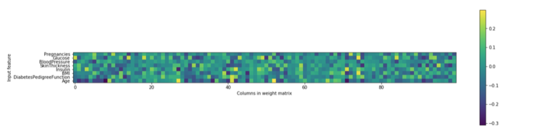
From the heat map, it is not easy to point out quickly that which feature (features) have relatively low weights compared to the other features.
Summary
We practiced a wide array of machine learning models for classification and regression, what their advantages and disadvantages are, and how to control model complexity for each of them. We saw that for many of the algorithms, setting the right parameters is important for good performance.
We should be able to know how to apply, tune, and analyze the models we practiced above. It’s your turn now! Try applying any of these algorithms to the built-in datasets in scikit-learn or any data set at your choice. Happy Machine Learning!
The source code that created this post can be found here. I would be pleased to receive feedback or questions on any of the above.
Reference: Introduction to Machine Learning with Python