Logistic Regression with Python using Titanic data

Near, far, wherever you are — That’s what Celine Dion sang in the Titanic movie soundtrack, and if you are near, far or wherever you are, you can follow this Python Machine Learning analysis by using the Titanic dataset provided by Kaggle.

We are going to make some predictions about this event. Let’s get started! First, find the dataset in Kaggle.

Let’s start by adding some libraries.

Panda’s is great for handling datasets, on the other hand, matplotlib and seaborn are libraries for graphics.

import pandas as pd
import matplotlib.pyplot as plt
import seaborn as sns
%matplotlib inline
Copy

We load the dataset.

train = pd.read_csv("train.csv")
Copy

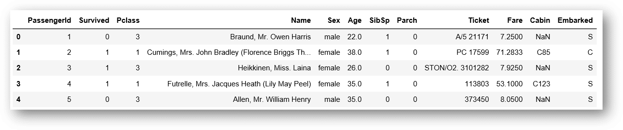
First, let’s see the data a little bit.

train.head()
Copy

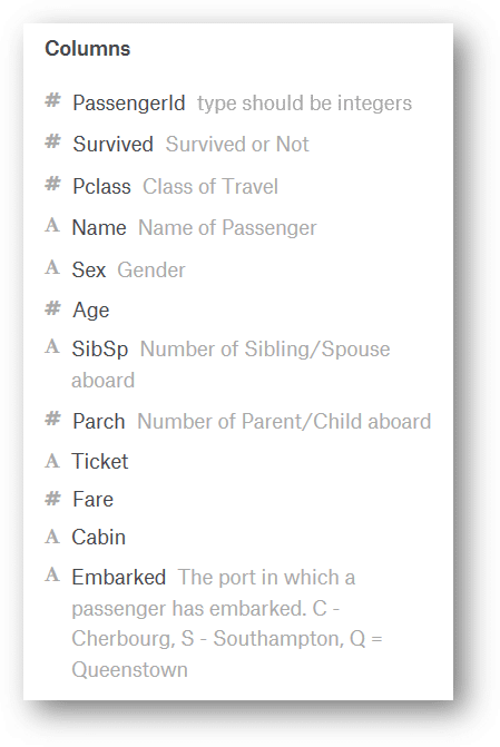
Here’s the Data Dictionary, so we can understand better the columns info:

As we can see here, the ship was very big, so there must be a lot of people there, let’s see how many people:

train.count()
Copy

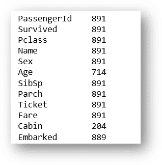
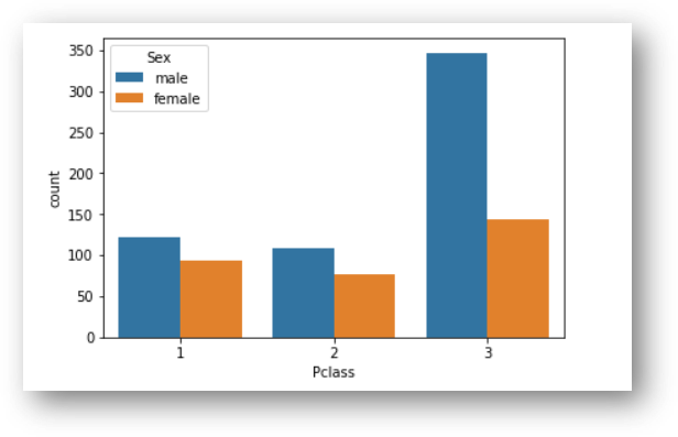
Ok, we can see 891 total. There are some null values for some columns, later we are going to deal with that. Let’s see how many men and women were there:

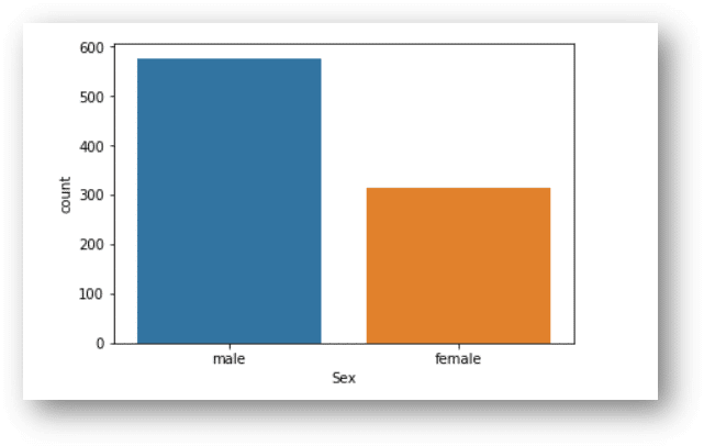
According to this graphic, we can see more men than women, let’s see how many exactly:

train[train['Sex'].str.match("female")].count()
Female: 314Copy

train[train['Sex'].str.match("male")].count()
Male: 577Copy

In the movie, we can see actors like Leonardo DiCaprio, Kate Winslet, and Kathy Bates. If you are interested in the full cast & crew, see this info: Titanic Cast & Crew

In the cast, we can see Leonardo DiCaprio character was Jack Dawson, Kate Winslet as Rose Dewitt Bukater and Kathy Bates as Molly Brown.
Let’s take a look at the names column to look for them:

train[train["Name"].str.contains("Dawson")]
No resultsCopy

train[train["Name"].str.contains("Bukater")]
No resultsCopy

train[train["Name"].str.contains("Brown")]
Click on the image below to see the resultCopy

Molly Brown was a real passenger in the Titanic. We can see more info about her on Wikipedia. If you read the Wikipedia article, you can find out she was a rich woman, no wonder she was traveling in class 1. We can see that most of the men were traveling in class 3 (that was the case of Jack Dawson in the movie).

Fortunately, Molly did survive. Let’s see how many people survived divided by class.

sns.countplot(x='Survived', hue='Pclass', data=train)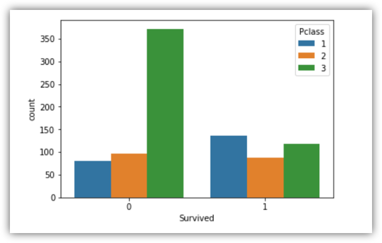
Copy

Let’s see how many people survived divided by sex.

sns.countplot(x='Survived', hue='Sex', data=train)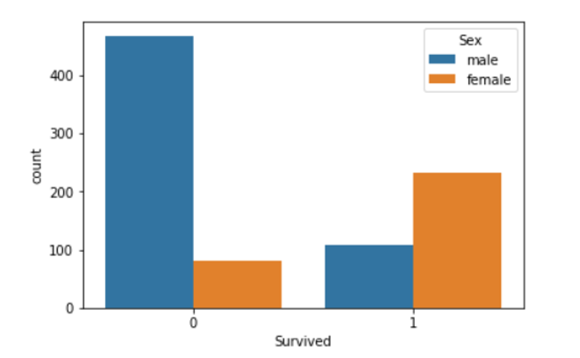
Copy

We can infer that, as Molly, if you were a female and you were in class 1, probably you would survive.
On the other hand, if you were a man and you were in class 3, you didn’t have good chances to live.

As we saw before, we have some null values for age. Let’s create a function to impute ages regarding the corresponding age average per class.

plt.figure(figsize=(10,7))
sns.boxplot(x='Pclass',y='Age',data=train)
Copy

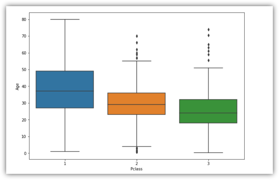
Let’s impute average age values to null age values:

def add_age(cols):
    Age = cols[0]
    Pclass = cols[1]
    if pd.isnull(Age):
        return int(train[train["Pclass"] == Pclass]["Age"].mean())
    else:
        return Age
Copy

Here, we call the function this way:

train["Age"] = train[["Age", "Pclass"]].apply(add_age,axis=1)
Copy

We have lots of null values for Cabin column, so we just remove it.

train.drop("Cabin",inplace=True,axis=1)
Copy

Finally, we remove some rows with null values:

train.dropna(inplace=True)
Copy

Ok, we are done with cleaning the data. We are going to convert some categorical data into numeric. For example, the sex column.

Let’s use the get_dummies function of Pandas. It will create two columns, one for male, one for female.

pd.get_dummies(train["Sex"])
Copy

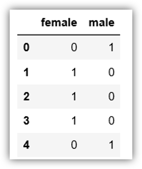
What we can do is to remove the first column because one column indicates the value of the other column.
For example, if the male is 1, then the female will be 0 and vice versa.

sex = pd.get_dummies(train["Sex"],drop_first=True)
Copy

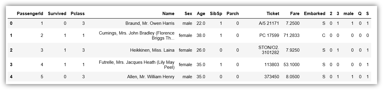
Let’s do the same for Embarked and PClass:

embarked = pd.get_dummies(train["Embarked"],drop_first=True)
embarked = pd.get_dummies(train["Pclass"],drop_first=True)
Copy

We add these variables to the dataset:

train = pd.concat([train,pclass,sex,embarked],axis=1)
Copy

Then, we remove some columns that we are not going to use for our model.

train.drop(["PassengerId","Pclass","Name","Sex","Ticket","Embarked"],axis=1,inplace=True)
Copy

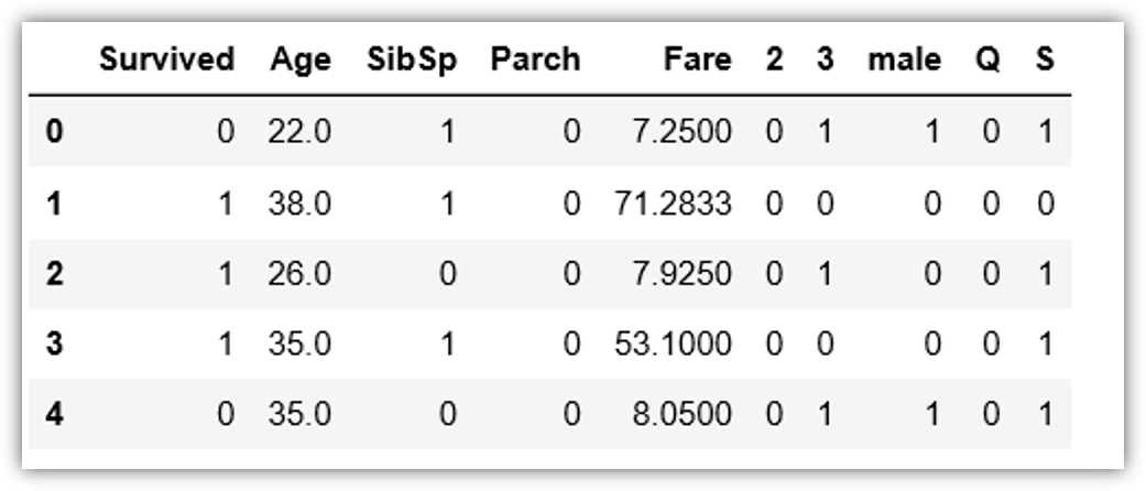
Now our dataset is ready for the model.

X will contain all the features and y will contain the target variable

X = train.drop("Survived",axis=1)
y = train["Survived"]
Copy

We will use train_test_split from cross_validation module to split our data. 70% of the data will be training data and %30 will be testing data.

from sklearn.cross_validation import train_test_split
X_train, X_test, y_train, y_test = train_test_split(X, y, test_size = 0.3, random_state = 101)
Copy

Let’s use Logistic Regression to train the model:

from sklearn.linear_model import LogisticRegression
logmodel = LogisticRegression()
logmodel.fit(X_train,y_train)
Copy

Let’s see how accurate is our model for predictions:

predictions = logmodel.predict(X_test)
from sklearn.metrics import classification_report
print(classification_report(y_test, predictions))
Copy

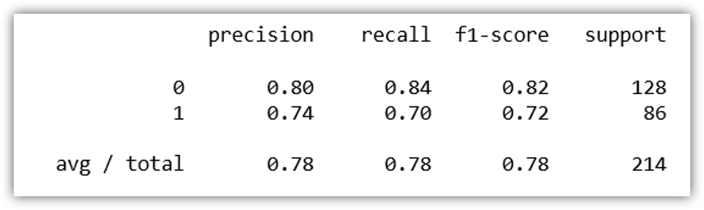
We got 78% accuraccy, not bad. Let’s see the confusion matrix

from sklearn.metrics import confusion_matrix
confusion_matrix(y_test, predictions)
Copy

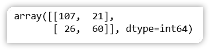
True positive: 107 (We predicted a positive result and it was positive)
True negative: 60 (We predicted a negative result and it was negative)
False positive: 21 (We predicted a positive result and it was negative)
False negative: 26 (We predicted a negative result and it was positive)

We still can improve our model, this tutorial is intended to show how we can do some exploratory analysis, clean up data, perform predictions and talk about this event and this wonderful movie.

Thanks!

Diego Lescano.

Logistic RegressionMachine Learning