Linear Mixed effect Models are becoming a common statistical tool for analyzing data with a multilevel structure. I will start by introducing the concept of multilevel modeling where we will see that such models are a compromise between two extreme: complete pooling and no pooling. Then I will present a typical workflow for the analysis of multilevel data using the package lme4 in R.
Mixed-effect models (or Multilevel modeling)
A multilevel structure is when the data are organized in different levels or groups, each with its own variation. For example say we measured the speed of reaction over repeated measurement on 50 people with varying sunlight. We might expect that some people will naturally be faster than others and so we need to include this in the model. A classical model would look like this (with j indexing the individuals between 1 and 50, and i indexing the observation between 1 and n):
$$Reaction_{ij}=\beta_{0}+\beta_{1}*Sunlight_{i}+\beta_{2}*(j=2)+..+\beta_{50}*(j=50)+\epsilon_{i}$$ $$ \epsilon_{i} \sim N(0,\sigma) $$
The \(j=X\) terms is returning 1 if the observation comes from the \(j_th\) person, 0 otherwise. You can clearly see two issues with such a model: (i) which individual is chosen to give the intercept \(\beta_{0}\)? There are most of the time no reason to put one instead of the other, as we would ensure that the individual monitored are a representative sample of the population under study. (ii) there are a lots of coefficient in this model (50+2) and empirical dataset are usually of “small” size leading to high uncertainties when the number of estimated coefficient is large relative to the sample size. This approach is called no pooling.
Another way to approach the data would be to completely ignore the grouping structure, this is called complete pooling and the model would look like:
$$Reaction_{i}=\beta_{0}+\beta_{1}*Sunlight_{i}+\epsilon_{i} $$ $$\epsilon_{i}\sim N(0,\sigma)$$
The complete pooling model ignore all variations between individuals and will gives the impression of having very precise (and so very significant) coefficients. In this case the assumption of independence of the residuals would be violated.
Mixed-effect models follow an approach between these two extreme, they will estimate the overall mean response (just like in complete pooling) but will add to it random deviation based on the grouping structure of the data (like in no pooling). The model would then look like this:
$$ Reaction_{ij} = \beta_{0} + \gamma_{j} + \beta_{1}*Sunlight_{i} + \epsilon_{i} $$ $$ \epsilon_{i} \sim N(0,\sigma_{residuals}) $$ $$ \gamma_{j} \sim N(0,\sigma_{individuals}) $$
This models will give for each individual an estimated deviation from the overall mean reaction time (the coefficient), so that the grouping structure of the data is taken into account while at the same time estimating (only) 4 coefficient when the no pooling model estimated 52 coefficient! Such a model can of course be extended with group-level variable like age or height, remember in this example the individuals are each forming one group of data, and the effect of such variables can be precisely modeled by taking into account both observation-level and group-level variations. Note that in all these models we assume a constant sunlight effect on reaction speed across individuals (ie no interaction individuals*sunlight). Enough theoretical consideration for now let’s dive in some concrete analysis.
Mixed-effect model in R
Let’s look at one simulated dataset to see how mixed-effect works in R:
#load libraries
library(lme4)
library(arm) #for the sim function
#simulate a dataset
set.seed(10)
#we measured plant biomass at 20 different sites with varying temperature and different nutrient levels
#we have 5 sample per sites
data<-data.frame(Temp=runif(100,-2,2),N=runif(100,-2,2),Site=gl(n=20,k=5,labels=paste0("Site",1:20)))
#some simulated parameters
params<-c(10,0.3,2.2)
rnd_int<-rnorm(20,0,1.2)
rnd_slp<-rnorm(20,0,0.5)
#the expected plant biomass
mus<-params[1]+rnd_int[data$Site]+(params[2]+rnd_slp[data$Site])*data$Temp+params[3]*data$N
#one simulation
data$Biomass<-rnorm(100,mus,1)
These simulated data have an intercept varying with the sites (we will get one estimation per site of the random deviation from the average plant biomass), similarly the slope of the effect of temperature on plant biomass also has a random deviate per site. The simulated model looks like this (for \(i = 1\), …, 100 observations and \(j = 1\), …, 20 sites):
$$Biomass_{ij} = \beta_{0} + \gamma_{j} + (\beta_{1} + \delta_{j})*Temperature_{i} + \beta_{2}*N_{i} + \epsilon_{i}$$ $$ \epsilon_{i} \sim N(0,\sigma_{residuals}) $$ $$ \gamma_{j} \sim N(0,\sigma_{sites\_intercept}) $$ $$ \delta_{j} \sim N(0,\sigma_{sites\_slope}) $$
Our model is called varying-intercept and varying-slope. To understand the varying-slope term, think about an interaction term between Temperature and Sites, the only difference is that instead of estimating the slope for each sites in isolation, the model will estimate the variation around the mean slope.
Model fitting
#fitting the models
m1<-lmer(Biomass~Temp+N+(1+Temp|Site),data)
Before going into the model output let’s briefly discuss the way to specify formula in lmer. The random terms (ie the varying-intercept) are given between parenthesis “()“, on the left-side of the “|” symbol come the terms that will vary between the groups. For example (1+Temp|Site) say that both the intercept and the Temp slope are varying between the sites. On the right-side of the “|” comes the grouping variable. Have a look here for a list of the different ways to set the random effect structure.
Model Checking
Remember from the equation before that the residuals must be normally distributed with constant standard deviation, this is like LM. One further assumption is that the random site effect must also be normally distributed. To check this we will plot the model residuals and the random effects:
par(mfrow=c(2,2))
plot(fitted(m1),resid(m1,type="pearson"),col="blue") #a plot to check the constant standard deviation
abline(h=0,lwd=2)
qqnorm(resid(m1)) #normality of the residuals
qqline(resid(m1))
qqnorm(ranef(m1)$Site[,1])
qqline(ranef(m1)$Site[,1])
qqnorm(ranef(m1)$Site[,2])
qqline(ranef(m1)$Site[,2])
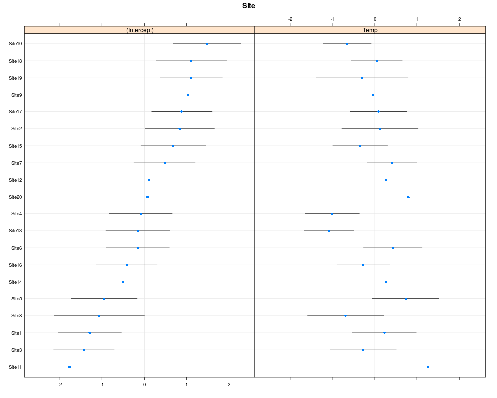
In the top-left graph one should see no pattern in the residuals, like stars in the sky. For the top-right one the point should fall more or less on the line. In the two bottom graph the points should also fall on the line, but note that in cases where the number of grouping level is low (<20) deviation from normality on these graphs should not lead to model rejection. One may also look at the random effect in a caterpillar plot:
library(lattice)
dotplot(ranef(m1,condVar=TRUE))
Inference
summary(m1)
Linear mixed model fit by REML ['lmerMod']
Formula: Biomass ~ Temp + N + (1 + Temp | Site)
   Data: data

REML criterion at convergence: 327.2

Scaled residuals:
     Min       1Q   Median       3Q      Max
-1.87964 -0.51590  0.03338  0.47663  1.84536

Random effects:
 Groups   Name        Variance Std.Dev. Corr
 Site     (Intercept) 1.0701   1.0345
          Temp        0.5089   0.7133   -0.20
 Residual             0.7681   0.8764
Number of obs: 100, groups:  Site, 20

Fixed effects:
            Estimate Std. Error t value
(Intercept)  10.0915     0.2509   40.23
Temp          0.1674     0.1904    0.88
N             2.2096     0.0944   23.41

Correlation of Fixed Effects:
     (Intr) Temp
Temp -0.123
N    -0.018  0.002
The model summary output gives you a lot of information, first is given some information on the model. Then comes some distribution statistic of the residuals, you want the residuals to be approximately symmetrically distributed, ie if the min is -1 but the max is 8 something is wrong. The residuals should also be centered around 0, ie a median more or less close to 0. Then comes the estimation of all the parameters, we see that σsites_intercept is estimated at 1.03, σsites_slope at 0.71 and finally σresiduals at 0.88. Which is not so bad considering that the simulated values are 1.2, 0.5 and 1.0. The next table gives us the estimated fixed-effect coefficient ie the β, together with their standard errors and a t-value.
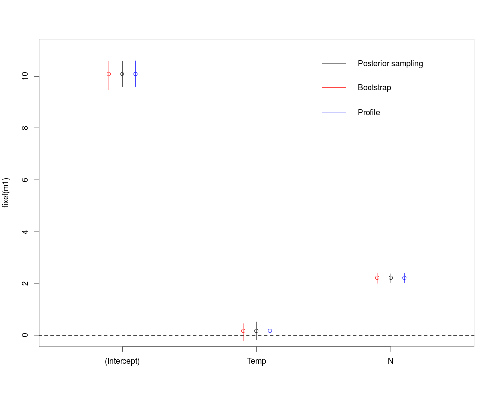
At this point most people using lmer for the first time are wondering where are the p-values, there is a long discussion on this issue, as always there are many approach to get them I will illustrate 3 of them based on confidence intervals below.
#different ways to get p-value for the fixed effects
#Credible intervals from posterior sampling
sims<-sim(m1,n.sims=200)
str(sims)
crI<-apply(sims@fixef,2,function(x) quantile(x,probs=c(0.025,0.975)))
plot(1:3,fixef(m1),ylim=c(0,11),xaxt="n",xlim=c(0.5,3.5),xlab="")
axis(1,at=1:3,labels=names(fixef(m1)))
segments(1:3,crI[1,],1:3,crI[2,])
abline(h=0,lty=2,lwd=2)
#bootstrap Confidence Intervals
boots<-confint(m1,parm=5:7,method="boot",nsim=200)
points((1:3)-0.1,fixef(m1),col="red")
segments((1:3)-0.1,boots[,1],(1:3)-0.1,boots[,2],col="red")
#profile Confidence Intervals
prof<-confint(m1,parm=5:7,method="profile")
points((1:3)+0.1,fixef(m1),col="blue")
segments((1:3)+0.1,prof[,1],(1:3)+0.1,prof[,2],col="blue")
legend("topright",legend=c("Posterior sampling","Bootstrap","Profile"),lwd=1,col=c("black","red","blue"),bty="n")
Formal class 'sim.merMod' [package "arm"] with 3 slots
  ..@ fixef: num [1:200, 1:3] 10.13 10.17 9.98 9.63 10.3 ...
  .. ..- attr(*, "dimnames")=List of 2
  .. .. ..$ : NULL
  .. .. ..$ : chr [1:3] "(Intercept)" "Temp" "N"
  ..@ ranef:List of 1
  .. ..$ Site: num [1:200, 1:20, 1:2] -1.053 -1.803 -1.136 -0.973 -1.711 ...
  .. .. ..- attr(*, "dimnames")=List of 3
  .. .. .. ..$ : NULL
  .. .. .. ..$ : chr [1:20] "Site1" "Site2" "Site3" "Site4" ...
  .. .. .. ..$ : chr [1:2] "(Intercept)" "Temp"
  ..@ sigma: num [1:200] 0.79 0.878 0.88 0.905 0.872 ...
The first method use the sim function which randomly draw posterior samples of the coefficients based on the fitted models. We can draw as many sample as we want and based on Bayesian theory the 0.025 and 0.975 quantiles of the sampled values will form the 95% credible intervals around the fitted value (the one we got from the model output). The second method will simulate new Biomass data from the given explanatory variables and the fitted models, it will then re-fit the model to these simulated response values and will extract the fitted coefficient. From this distribution of bootstrapped coefficient it will draw a 95% confidence interval around the fitted values. Finally the third method will compute profile likelihood value and will determine when are these profile likelihood values not significantly different from the profile likelihood you would get if the parameter of interest was set to 0. This will also gives a 95% confidence interval. As always in R there are many ways to get what you want (one could also use the package lmerTest or afex), based on your data you may choose which one to use.
Plotting the results
#plot Temp effects
new_temp<-data.frame(Temp=seq(-2,2,length=20),N=mean(data$N))
pred_temp<-predict(m1,newdata=new_temp,re.form=~0)
#compute bootstrapped confidence interval, see ?predict.merMod
ci_line<-bootMer(m1,FUN=function(.) predict(.,newdata=new_temp,re.form=~0),nsim=200)
ci_regT<-apply(ci_line$t,2,function(x) x[order(x)][c(5,195)])
par(mfrow=c(1,2))
plot(Biomass~Temp,data)
lines(new_temp$Temp,pred_temp,lwd=3)
lines(new_temp$Temp,ci_regT[1,],lty=2)
lines(new_temp$Temp,ci_regT[2,],lty=2)
#for N effects
new_n<-data.frame(Temp=mean(data$Temp),N=seq(-2,2,length=20))
pred_n<-predict(m1,newdata=new_n,re.form=~0)
ci_line<-bootMer(m1,FUN=function(.) predict(.,newdata=new_n,re.form=~0),nsim=200)
ci_regN<-apply(ci_line$t,2,function(x) x[order(x)][c(5,195)])
plot(Biomass~N,data)
lines(new_n$N,pred_n,lwd=3)
lines(new_n$N,ci_regN[1,],lty=2)
lines(new_n$N,ci_regN[2,],lty=2)
mtext(text="Regression curves with 95% confidence intervals",side=3,outer=FALSE,at=-3)
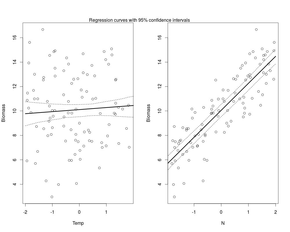
Note that you could also easily compute the credible interval around the regression line using the posterior draw from the model coefficient. Hopefully with all this material you should be able to apply linear mixed effect models to your data and to derive the usual information from these models. A few words of caution before the end: LMM are made for dataset when the number of levels grouping factor(s) is not too small (a rule of thumb is bigger than 5), models may fit to your data with only two levels in the grouping factor but in this case the estimated standard deviation and random effects will be imprecise. So in this case I would recommend to stick with LMs with no pooling. Overfitting your data can be a big issue if you do not have enough information in your dataset, so think carefully about what your model means, simulate some data from it, fit them with the models and see if you get what you would expect.
Reference
A great book to dive into multilevel modelling is Gelman and Hill 2007, the lme4 mailing list is also of great help if you have question or just want to browse through the archives. Update: You also might want to check out this great package implementing most of the workflow into nice functions and allowing to look at the models with a Shiny interface,


