Note: This article has since been updated. More recent and up-to-date findings can be found at: Regression-based neural networks: Predicting Average Daily Rates for Hotels
Keras is an API used for running high-level neural networks. The model runs on top of TensorFlow, and was developed by Google.
The main competitor to Keras at this point in time is PyTorch, developed by Facebook. While PyTorch has a somewhat higher level of community support, it is a particularly verbose language and I personally prefer Keras for greater simplicity and ease of use in building and deploying models.
In this particular example, a neural network will be built in Keras to solve a regression problem, i.e. one where our dependent variable (y) is in interval format and we are trying to predict the quantity of y with as much accuracy as possible.
What Is A Neural Network?
A neural network is a computational system that creates predictions based on existing data. Let us train and test a neural network using the neuralnet library in R.
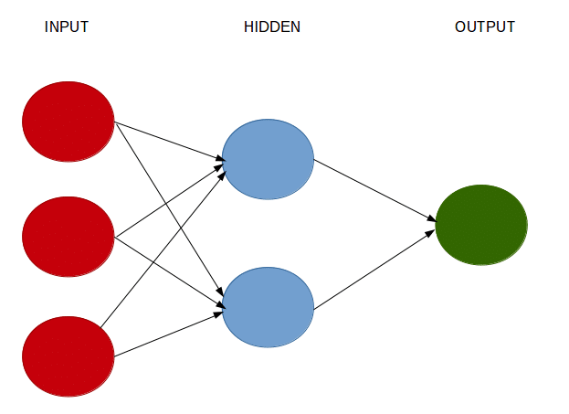
A neural network consists of:
- Input layers: Layers that take inputs based on existing data
- Hidden layers: Layers that use backpropagation to optimise the weights of the input variables in order to improve the predictive power of the model
- Output layers: Output of predictions based on the data from the input and hidden layers
Our Example
For this example, we use a linear activation function within the keras library to create a regression-based neural network. We will use the cars dataset. Essentially, we are trying to predict the value of a potential car sale (i.e. how much a particular person will spend on buying a car) for a customer based on the following attributes:
- Age
- Gender
- Average miles driven per day
- Personal debt
- Monthly income
Firstly, we import our libraries. Note that you will need TensorFlow installed on your system to be able to execute the below code. Depending on your operating system, you can find one of my YouTube tutorials on how to install on Windows 10 here.
Libraries
import matplotlib.pyplot as plt
import numpy as np
import pandas as pd
from sklearn.model_selection import train_test_split
from sklearn.model_selection import cross_val_score
from sklearn.model_selection import KFold
from sklearn.pipeline import Pipeline
from sklearn.preprocessing import MinMaxScaler
from tensorflow.python.keras.models import Sequential
from tensorflow.python.keras.layers import Dense
from tensorflow.python.keras.wrappers.scikit_learn import KerasRegressor
Set Directory
import os;
path="C:/yourdirectory"
os.chdir(path)
os.getcwd()
Since we are implementing a neural network, the variables need to be normalized in order for the neural network to interpret them properly. Therefore, our variables are transformed using the MaxMinScaler():
#Variables
dataset=np.loadtxt("cars.csv", delimiter=",")
x=dataset[:,0:5]
y=dataset[:,5]
y=np.reshape(y, (-1,1))
scaler_x = MinMaxScaler()
scaler_y = MinMaxScaler()
print(scaler_x.fit(x))
xscale=scaler_x.transform(x)
print(scaler_y.fit(y))
yscale=scaler_y.transform(y)
The data is then split into training and test data:
X_train, X_test, y_train, y_test = train_test_split(xscale, yscale)
Keras Model Configuration: Neural Network API
Now, we train the neural network. We are using the five input variables (age, gender, miles, debt, and income), along with two hidden layers of 12 and 8 neurons respectively, and finally using the linear activation function to process the output.
model = Sequential()
model.add(Dense(12, input_dim=5, kernel_initializer='normal', activation='relu'))
model.add(Dense(8, activation='relu'))
model.add(Dense(1, activation='linear'))
model.summary()
The mean_squared_error (mse) and mean_absolute_error (mae) are our loss functions – i.e. an estimate of how accurate the neural network is in predicting the test data. We can see that with the validation_split set to 0.2, 80% of the training data is used to test the model, while the remaining 20% is used for testing purposes.
model.compile(loss='mse', optimizer='adam', metrics=['mse','mae'])
From the output, we can see that the more epochs are run, the lower our MSE and MAE become, indicating improvement in accuracy across each iteration of our model.
Neural Network Output
Let’s now fit our model.
>>> history = model.fit(X_train, y_train, epochs=150, batch_size=50,  verbose=1, validation_split=0.2)

Train on 577 samples, validate on 145 samples
Epoch 1/150
2019-06-01 22:44:17.138641: I tensorflow/core/platform/cpu_feature_guard.cc:141] Your CPU supports instructions that this TensorFlow binary was not compiled to use: AVX2 FMA
 50/577 [=>............................] - ETA: 12s - loss: 0.2160 - mean_square577/577 [==============================] - 1s 2ms/step - loss: 0.1803 - mean_squared_error: 0.1803 - mean_absolute_error: 0.3182 - val_loss: 0.1392 - val_mean_squared_error: 0.1392 - val_mean_absolute_error: 0.2688
Epoch 2/150
 50/577 [=>............................] - ETA: 0s - loss: 0.1373 - mean_squared577/577 [==============================] - 0s 54us/step - loss: 0.1279 - mean_squared_error: 0.1279 - mean_absolute_error: 0.2652 - val_loss: 0.0934 - val_mean_squared_error: 0.0934 - val_mean_absolute_error: 0.2287
Epoch 3/150
 50/577 [=>............................] - ETA: 0s - loss: 0.0790 - mean_squared577/577 [==============================] - 0s 56us/step - loss: 0.0850 - mean_squared_error: 0.0850 - mean_absolute_error: 0.2271 - val_loss: 0.0674 - val_mean_squared_error: 0.0674 - val_mean_absolute_error: 0.2147
Epoch 4/150
 50/577 [=>............................] - ETA: 0s - loss: 0.0739 - mean_squared577/577 [==============================] - 0s 51us/step - loss: 0.0640 - mean_squared_error: 0.0640 - mean_absolute_error: 0.2152 - val_loss: 0.0595 - val_mean_squared_error: 0.0595 - val_mean_absolute_error: 0.2123
Epoch 5/150
 50/577 [=>............................] - ETA: 0s - loss: 0.0661 - mean_squared577/577 [==============================] - 0s 53us/step - loss: 0.0559 - mean_squared_error: 0.0559 - mean_absolute_error: 0.2065 - val_loss: 0.0544 - val_mean_squared_error: 0.0544 - val_mean_absolute_error: 0.2042
...
Epoch 145/150
 50/577 [=>............................] - ETA: 0s - loss: 0.0100 - mean_squared577/577 [==============================] - 0s 53us/step - loss: 0.0127 - mean_squared_error: 0.0127 - mean_absolute_error: 0.0822 - val_loss: 0.0090 - val_mean_squared_error: 0.0090 - val_mean_absolute_error: 0.0732
Epoch 146/150
 50/577 [=>............................] - ETA: 0s - loss: 0.0189 - mean_squared577/577 [==============================] - 0s 56us/step - loss: 0.0128 - mean_squared_error: 0.0128 - mean_absolute_error: 0.0815 - val_loss: 0.0092 - val_mean_squared_error: 0.0092 - val_mean_absolute_error: 0.0749
Epoch 147/150
 50/577 [=>............................] - ETA: 0s - loss: 0.0172 - mean_squared577/577 [==============================] - 0s 55us/step - loss: 0.0126 - mean_squared_error: 0.0126 - mean_absolute_error: 0.0813 - val_loss: 0.0090 - val_mean_squared_error: 0.0090 - val_mean_absolute_error: 0.0737
Epoch 148/150
 50/577 [=>............................] - ETA: 0s - loss: 0.0105 - mean_squared577/577 [==============================] - 0s 60us/step - loss: 0.0127 - mean_squared_error: 0.0127 - mean_absolute_error: 0.0812 - val_loss: 0.0092 - val_mean_squared_error: 0.0092 - val_mean_absolute_error: 0.0748
Epoch 149/150
 50/577 [=>............................] - ETA: 0s - loss: 0.0148 - mean_squared577/577 [==============================] - 0s 52us/step - loss: 0.0127 - mean_squared_error: 0.0127 - mean_absolute_error: 0.0827 - val_loss: 0.0089 - val_mean_squared_error: 0.0089 - val_mean_absolute_error: 0.0730
Epoch 150/150
 50/577 [=>............................] - ETA: 0s - loss: 0.0121 - mean_squared577/577 [==============================] - 0s 52us/step - loss: 0.0128 - mean_squared_error: 0.0128 - mean_absolute_error: 0.0821 - val_loss: 0.0090 - val_mean_squared_error: 0.0090 - val_mean_absolute_error: 0.0737
Here, we can see that keras is calculating both the training loss and validation loss, i.e. the deviation between the predicted y and actual y as measured by the mean squared error.
As you can see, we have specified 150 epochs for our model. This means that we are essentially training our model over 150 forward and backward passes, with the expectation that our loss will decrease with each epoch, meaning that our model is predicting the value of y more accurately as we continue to train the model.
Let’s see what this looks like when we plot our respective losses:
print(history.history.keys())
# "Loss"
plt.plot(history.history['loss'])
plt.plot(history.history['val_loss'])
plt.title('model loss')
plt.ylabel('loss')
plt.xlabel('epoch')
plt.legend(['train', 'validation'], loc='upper left')
plt.show()
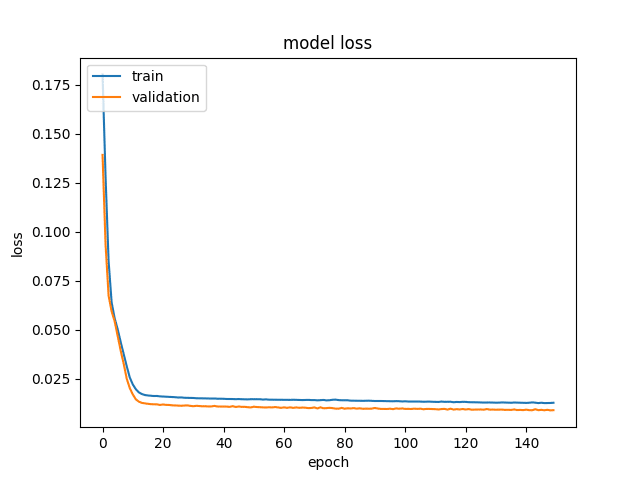
Both the training and validation loss decrease in an exponential fashion as the number of epochs is increased, suggesting that the model gains a high degree of accuracy as our epochs (or number of forward and backward passes) is increased.
Predictions
So, we’ve seen how we can train a neural network model, and then validate our training data against our test data in order to determine the accuracy of our model.
However, what if we now wish to use the model to estimate unseen data?
Let’s take the following array as an example:
Xnew = np.array([[40, 0, 26, 9000, 8000]])
Using this data, let’s plug in the new values to see what our calculated figure for car sales would be:
Xnew = np.array([[40, 0, 26, 9000, 8000]])
Xnew= scaler_x.transform(Xnew)
ynew= model.predict(Xnew)
#invert normalize
ynew = scaler_y.inverse_transform(ynew)
Xnew = scaler_x.inverse_transform(Xnew)
print("X=%s, Predicted=%s" % (Xnew[0], ynew[0]))
X=[  40.    0.   26. 9000. 8000.], Predicted=[13686.491]
Conclusion
In this tutorial, you have learned how to:
- Construct neural networks with Keras
- Scale data appropriately with MinMaxScaler
- Calculate training and test losses
- Make predictions using the neural network model
Many thanks for your time.