In this post, we’ll explore how Monte Carlo simulations can be applied in practice. In particular, we will see how we can run a simulation when trying to predict the future stock price of a company. There is a video at the end of this post which provides the Monte Carlo simulations. You can get the basics of Python by reading my other post Python Functions for Beginners.
There is a group of libraries and modules that can be imported when carrying out this task. Besides the classical NumPy and Pandas, we will need “norm” from SciPy and some specific Matplotlib features.
import numpy as np
import pandas as pd
from pandas_datareader import data as wb
import matplotlib.pyplot as plt
from scipy.stats import norm
%matplotlib inline
The company we will use for our analysis will be P&G. The timeframe under consideration reflects the past 10 years, starting from January the 1st 2007.
ticker = 'PG'
data = pd.DataFrame()
data[ticker] = wb.DataReader(ticker, data_source='yahoo', start='2007-1-1')['Adj Close']
We want to forecast P&G’s future stock price in this exercise. So, the first thing we’ll do is estimate its historical log returns. The method we’ll apply here is called “percent change”, and you must write “pct_change()” to obtain the simple returns from a provided dataset. We can create the formula for log returns by using NumPy’s log and then type 1 + the simple returns extracted from our data. And… here’s a table with P&G’s log returns.
log_returns = np.log(1 + data.pct_change())
log_returns.tail()
	PG
Date
2017-04-04	0.002561
2017-04-05	0.000667
2017-04-06	-0.006356
2017-04-07	-0.001903
2017-04-10	0.002910
Awesome!
data.plot(figsize=(10, 6));
Gives this plot:
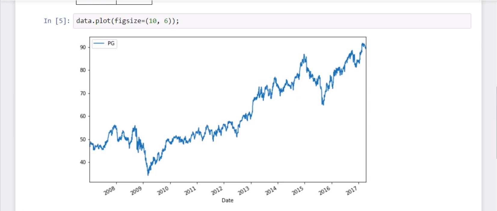
In the first graph, we can see P&G’s price, which has been gradually growing during the past decade.
log_returns.plot(figsize = (10, 6))
Gives this plot:
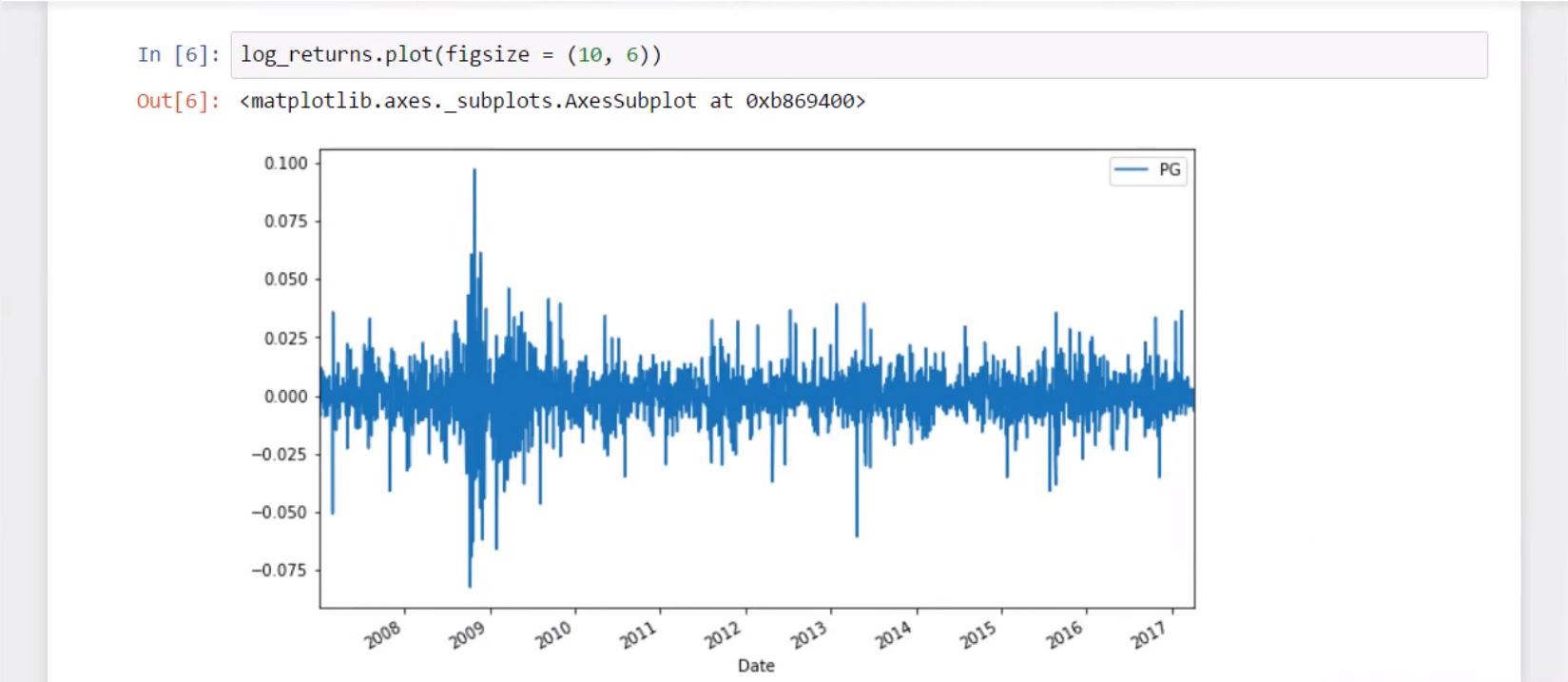
In the second one, we plot the log returns, not the price, of P&G. The picture tells us the returns are normally distributed and have a stable mean. Great!
Now, let’s explore their mean and variance, as we will need them for the calculation of the Brownian motion.
We need to know how to calculate mean and variance.
After a few lines of code, we obtain these numbers.
u = log_returns.mean()
u
PG    0.000244
dtype: float64
var = log_returns.var()
var
PG    0.000124
dtype: float64
So… what are we going to do with them?
First, I’ll compute the drift component. It is the best approximation of future rates of return of the stock. The formula to use here will be “U”, which equals the average log return, minus half its variance.
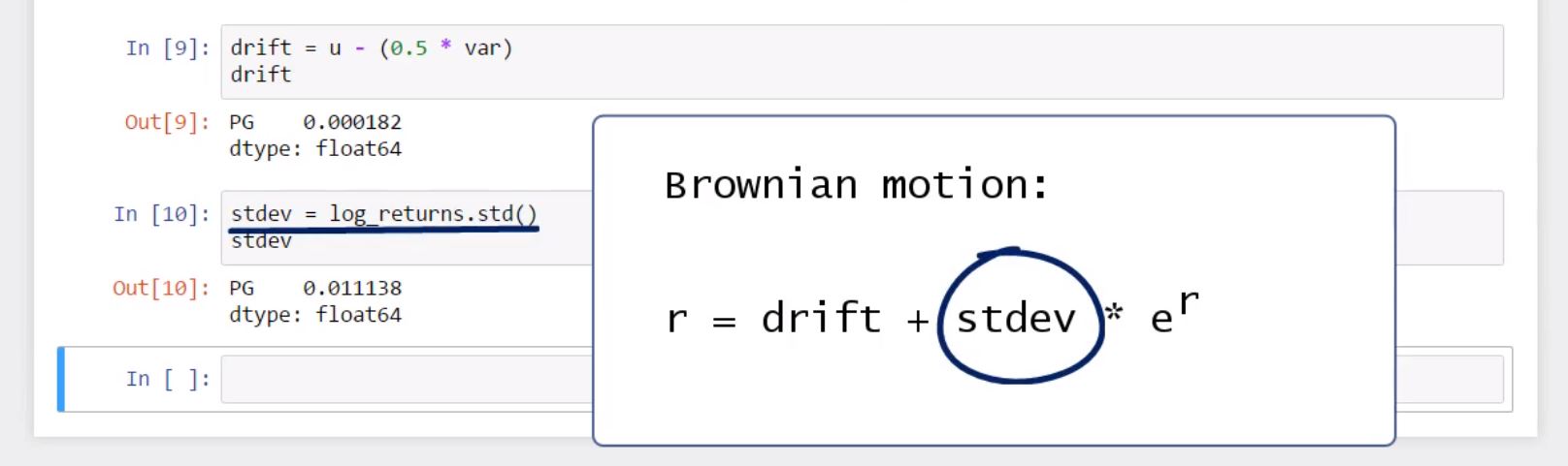
drift = u - (0.5 * var)
drift
PG    0.000182
dtype: float64
All right! We obtained a tiny number, and that need not scare you, because we’ll do this entire exercise without annualizing our indicators. Why? Because we will try to predict P&G’s daily stock price. Good!
Next, we will create a variable, called “stdev”, and we will assign to it the standard deviation of log returns. We said the Brownian motion comprises the sum of the drift and a variance adjusted by “E” to the power of “R”, so we will use this block in the second part of the expression.
stdev = log_returns.std()
stdev
PG    0.011138
dtype: float64
Ok. We’ve set up the first Brownian motion element in our simulation.
Next, we will create the second component and will show you how this would allow us to run a simulation about a firm’s future stock price.
Until now, we obtained the “drift” and standard deviation values we will need for the calculation of daily returns. The “type” function allows us to check their type and see it is Pandas Series.
type(drift)
pandas.core.series.Series
type(stdev)
pandas.core.series.Series
To proceed with our task, we should convert these values into NumPy arrays.
You already know the NumPy’s array method can do this for us. However, let me demonstrate how typing “dot values” after a Pandas object, be it a series or a data frame, can transfer the object into a NumPy array.
np.array(drift)
array([ 0.00018236])
drift.values
array([ 0.00018236])
You see? We obtain the same output for the drift as we did with “NumPy dot array”!
Then, “stdev.values” provides an analogical output and allows us to obtain the standard deviation. Great!
stdev.values
array([ 0.0111381])
The second component of the Brownian motion is a random variable, z, a number corresponding to the distance between the mean and the events, expressed as the number of standard deviations.
SciPy’s norm dot “PPF” allows us to obtain this result.
norm.ppf(0.95)
1.6448536269514722
If an event has a 95% chance of occurring, the distance between this event and the mean will be approximately 1.65 standard deviations, ok? This is how it works.
To complete the second component, we will need to randomize. The well-known NumPy “rand” function can help us do that easily. If we want to create a multi-dimensional array, we will need to insert two arguments. So, I’ll type 10 and 2.
x = np.random.rand(10, 2)
x
array([[ 0.86837673,  0.64121587],
       [ 0.35250561,  0.76738945],
       [ 0.56417914,  0.76087099],
       [ 0.8227844 ,  0.84426587],
       [ 0.19938002,  0.48545445],
       [ 0.19256769,  0.17927412],
       [ 0.74112595,  0.28645219],
       [ 0.54068474,  0.75853205],
       [ 0.21367244,  0.80188773],
       [ 0.92836315,  0.29874961]])
Here you go! We obtained a 10 by 2 matrix.
We will include this random element within the “PPF” distribution to obtain the distance from the mean corresponding to each of these randomly generated probabilities. The first number from the first row corresponds to the first probability from the first row of the X matrix, the second element – to the second probability, as shown in the X matrix, and so on.
norm.ppf(x)
array([[ 1.11875061,  0.36171067],
       [-0.3785646 ,  0.73027664],
       [ 0.16157351,  0.7091071 ],
       [ 0.92602843,  1.01214599],
       [-0.84383782, -0.03646838],
       [-0.86847311, -0.91813491],
       [ 0.64682054, -0.56377924],
       [ 0.10215894,  0.70158838],
       [-0.79374333,  0.8483833 ],
       [ 1.46370816, -0.52800017]])
Great!
The whole expression corresponding to “Z” will be of the type
norm.ppf(np.random.rand(10,2)).
Z = norm.ppf(np.random.rand(10,2))
Z
array([[-0.06864316,  0.46165842],
       [-1.608198  ,  1.5847175 ],
       [-2.28620036, -0.68382222],
       [-0.83235356, -0.61163297],
       [ 0.56875206, -0.64247376],
       [ 0.02273682,  0.15843913],
       [-2.31777044, -0.62447944],
       [-1.12842234,  0.84162461],
       [ 0.78017813,  1.82510123],
       [ 0.66502436,  0.995354  ]])
The newly created array used the probabilities generated by the “rand” function and converted them into distances from the mean 0, as measured by the number of standard deviations. This expression will create the value of Z, as defined in our formula.
Cool!
So, once we have built these tools and calculated all necessary variables, we are ready to calculate daily returns. All the infrastructure is in place.
Ok. So, first, I would like to specify the time intervals we will use will be 1,000, because we are interested in forecasting the stock price for the upcoming 1,000 days. Then, to “iterations” I will attribute the value of 10, which means I will ask the computer to produce 10 series of future stock price predictions.
t_intervals = 1000
iterations = 10
Ok.
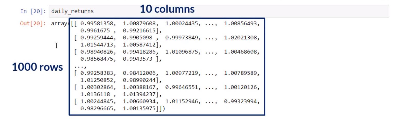
The variable “daily returns” will show us what will equal “E” to the power of “R”. We will need NumPy’s “EXP” function, which means we are calculating Euler’s number “E” raised to the power of the expression written between the parentheses.
daily_returns = np.exp(drift.values + stdev.values * norm.ppf(np.random.rand(t_intervals, iterations)))
In the parentheses, we will have the value of the drift and the product of the standard deviation and the random component, created with the help of the “norm” module. Its percentage value was generated with NumPy’s “rand” function, using “time intervals” and “iterations” specifying the dimensions of the array filled with values from 0 to 1.
daily_returns
array([[ 0.97303642,  0.97840622,  1.00789324, ...,  0.9907001 ,
         0.998585  ,  1.01371959],
       [ 1.0212853 ,  1.00158374,  1.00778714, ...,  0.99852295,
         1.00047002,  0.98616375],
       [ 1.014873  ,  1.00158135,  1.00964146, ...,  1.00443701,
         1.00555821,  0.99301348],
       ...,
       [ 1.02379495,  0.9767779 ,  0.97499868, ...,  0.99758644,
         1.0121379 ,  1.01268496],
       [ 0.9967678 ,  1.02578401,  0.99373039, ...,  0.99437147,
         1.00354653,  1.0042182 ],
       [ 1.01287017,  0.99566178,  0.9811977 , ...,  0.99093491,
         0.99359816,  0.97974084]])
Great!
So, the formula we used in the previous cell would allow us to obtain a 1,000 by 10 array with daily return values – 10 sets of 1,000 random future stock prices.
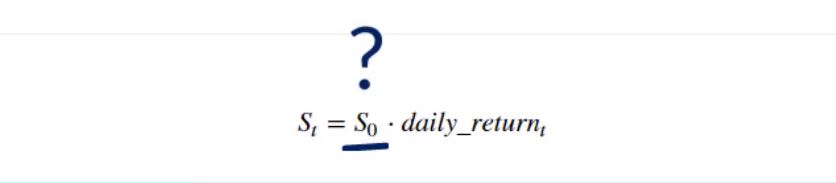
We are a single step away from completing this exercise. All we have to do is create a price list. Each price must equal the product of the price observed the previous day and the simulated daily return. Therefore, once we obtain the price in day T, we can estimate the expected stock price we will have in day T plus 1.

Then, this process will be repeated 1,000 times, and we will obtain a prediction of a company’s stock price 1,000 days from now.

This sounds awesome, but where can we start? We already created a matrix containing daily returns, right? So the daily returns variable is available.

However, which will be the first price in our list? 0? 1 million? Of course, not.
To make credible predictions about the future, the first stock price in our list must be the last one in our data set. It is the current market price. Let’s call this variable “S zero”, as it contains the stock price today (at the starting point, time 0). With the help of the “i-loc” method and the index operator, we can indicate we need the last value from the table by typing minus 1 within the brackets.
S0 = data.iloc[-1]
S0
PG    89.489998
Name: 2017-04-10 00:00:00, dtype: float64
Perfect! This is the first stock price on our list.
Let’s proceed with filling in the list. How big should it be? As big as the “daily returns” array, right?
This is why the price list matrix could be, at most, as big as the ‘daily returns’ matrix. And, as we all hoped, NumPy has a method that can create an array with the same dimensions as an array that exists and that we have specified.
This method is called “zeros like”. As an argument, insert the “daily returns” array.
price_list = np.zeros_like(daily_returns)
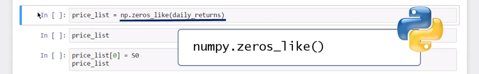
We will obtain an array of 1,000 by 10 elements, just like the dimension of “daily returns”, and then fill it with zeros.
price_list
array([[ 0.,  0.,  0., ...,  0.,  0.,  0.],
       [ 0.,  0.,  0., ...,  0.,  0.,  0.],
       [ 0.,  0.,  0., ...,  0.,  0.,  0.],
       ...,
       [ 0.,  0.,  0., ...,  0.,  0.,  0.],
       [ 0.,  0.,  0., ...,  0.,  0.,  0.],
       [ 0.,  0.,  0., ...,  0.,  0.,  0.]])
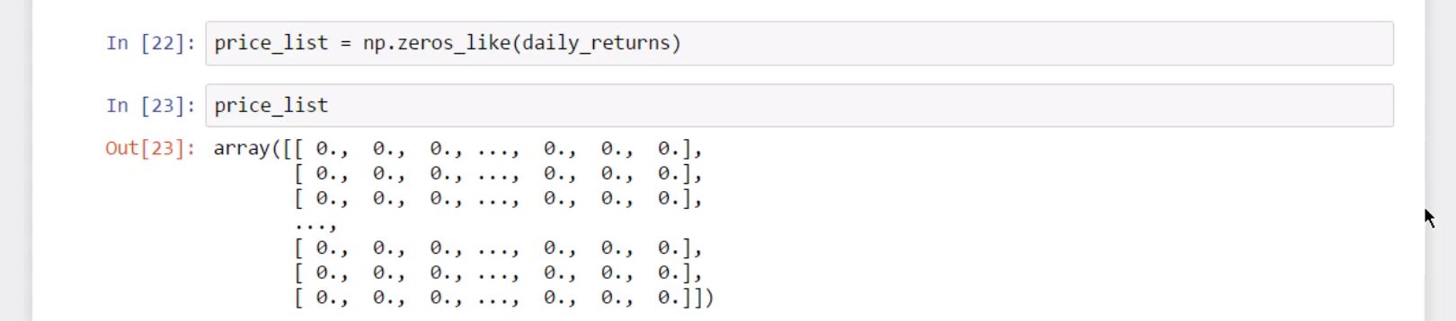
So, why did we create this object? Well, now we can replace these zeros with the expected stock prices by using a loop.
Let’s do this!
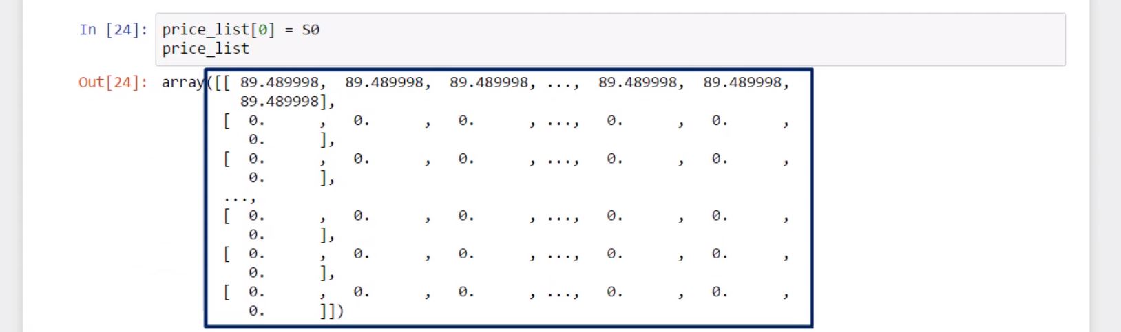
First, we must set the first row of our price list to “S zero”.
price_list[0]
array([ 0.,  0.,  0.,  0.,  0.,  0.,  0.,  0.,  0.,  0.])
Yes, not just the first value, but the entire row of 10 elements, because “S zero” will be the initial price for each of the 10 iterations we intend to generate. We will obtain the following array.
price_list[0] = S0
price_list
array([[ 89.489998,  89.489998,  89.489998, ...,  89.489998,  89.489998,
         89.489998],
       [  0.      ,   0.      ,   0.      , ...,   0.      ,   0.      ,
          0.      ],
       [  0.      ,   0.      ,   0.      , ...,   0.      ,   0.      ,
          0.      ],
       ...,
       [  0.      ,   0.      ,   0.      , ...,   0.      ,   0.      ,
          0.      ],
       [  0.      ,   0.      ,   0.      , ...,   0.      ,   0.      ,
          0.      ],
       [  0.      ,   0.      ,   0.      , ...,   0.      ,   0.      ,
          0.      ]])
Great!
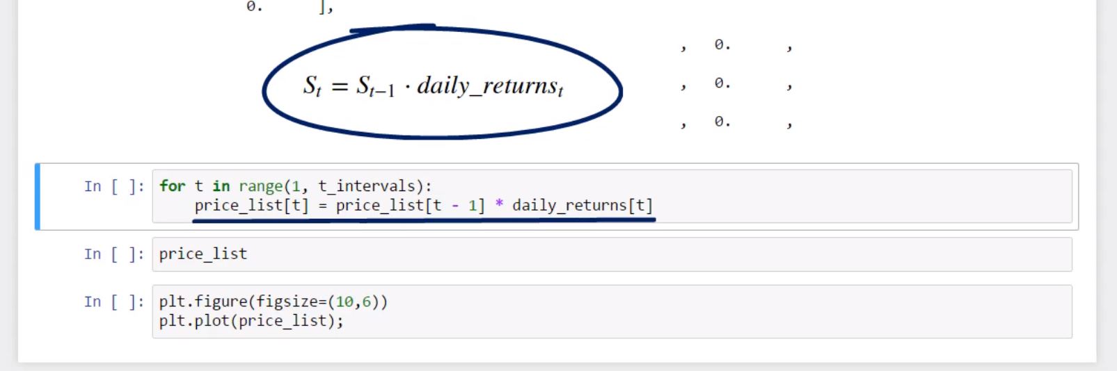
Finally, we can generate values for our price list. We must set up a loop that begins in day 1 and ends at day 1,000. We can simply write down the formula for the expected stock price on day T in Pythonic. It will be equal to the price in day T minus 1, times the daily return observed in day T.
for t in range(1, t_intervals):
    price_list[t] = price_list[t - 1] * daily_returns[t]
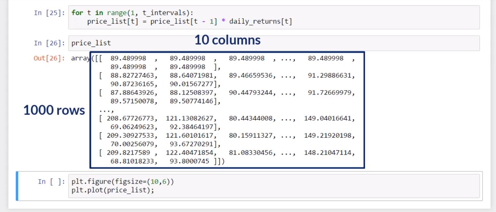
Let’s verify if we completed the price list.
Absolutely! See?
price_list
array([[  89.489998  ,   89.489998  ,   89.489998  , ...,   89.489998  ,
          89.489998  ,   89.489998  ],
       [  91.39481931,   89.63172707,   90.18686916, ...,   89.35781712,
          89.53206007,   88.25179158],
       [  92.75413425,   89.77346583,   91.05640268, ...,   89.75429866,
          90.02969795,   87.63521903],
       ...,
       [ 103.75544725,  160.47532431,   89.95735942, ...,   87.58142573,
         118.42781094,  161.60337685],
       [ 103.42008913,  164.61302111,   89.39336176, ...,   87.08847145,
         118.84781885,  162.28505283],
       [ 104.75112292,  163.89889345,   87.7125613 , ...,   86.29900685,
         118.08697415,  158.99729339]])
And if we would like to plot it on a graph with size 10 to 6, we can do that by using the Matplotlib syntax. When we execute, we will obtain 10 possible paths of the expected stock price of Procter and Gamble stock, starting from the last day for which we have data from yahoo. We called these trends iterations, since the computer will iterate through the provided formula 10 times.
Here, we have the paths we simulated.
plt.figure(figsize=(10,6))
plt.plot(price_list);
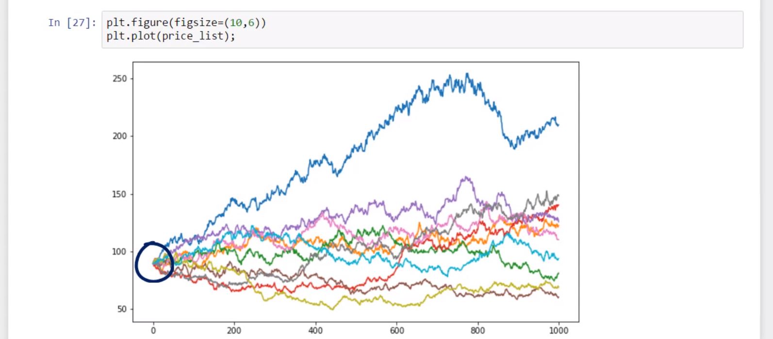
Amazing! Right?
This was another toughie, wasn’t it? We realize we got involved in more technical language and more advanced concepts, but this is the type of topics you need to master to get into the field of finance or data science.
Rewind if you would like to see how the process was carried out.
Thank you for reading!