Drawing a line through a cloud of point (ie doing a linear regression) is the most basic analysis one may do. It is sometime fitting well to the data, but in some (many) situations, the relationships between variables are not linear. In this case one may follow three different ways: (i) try to linearize the relationship by transforming the data, (ii) fit polynomial or complex spline models to the data or (iii) fit non-linear functions to the data. As you may have guessed from the title, this post will be dedicated to the third option.
What is non-linear regression?
In non-linear regression the analyst specify a function with a set of parameters to fit to the data. The most basic way to estimate such parameters is to use a non-linear least squares approach (function nls in R) which basically approximate the non-linear function using a linear one and iteratively try to find the best parameter values (wiki). A nice feature of non-linear regression in an applied context is that the estimated parameters have a clear interpretation (Vmax in a Michaelis-Menten model is the maximum rate) which would be harder to get using linear models on transformed data for example.
Fit non-linear least squares
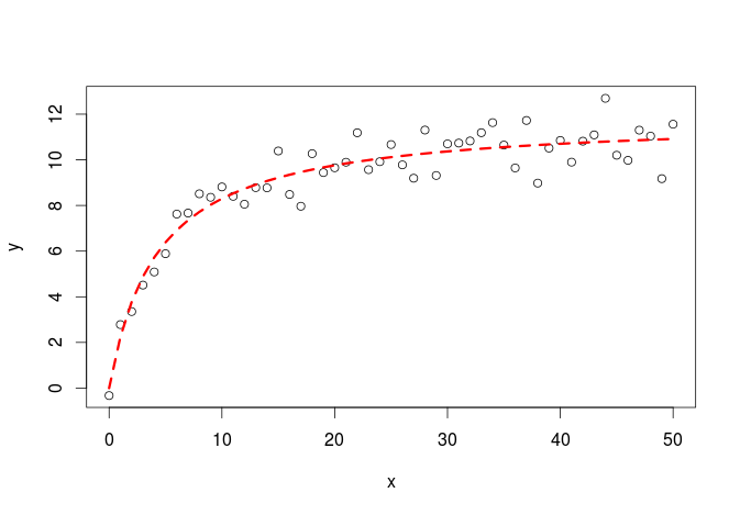
First example using the Michaelis-Menten equation:
#simulate some data
set.seed(20160227)
x<-seq(0,50,1)
y<-((runif(1,10,20)*x)/(runif(1,0,10)+x))+rnorm(51,0,1)
#for simple models nls find good starting values for the parameters even if it throw a warning
m<-nls(y~a*x/(b+x))
#get some estimation of goodness of fit
cor(y,predict(m))
[1] 0.9496598
Code below is to make a plot:
#plot
plot(x,y)
lines(x,predict(m),lty=2,col="red",lwd=3)
Here it is the plot:
The issue of finding the right starting values
Finding good starting values is very important in non-linear regression to allow the model algorithm to converge. If you set starting parameters values completely outside of the range of potential parameter values the algorithm will either fail or it will return non-sensical parameter like for example returning a growth rate of 1000 when the actual value is 1.04.
The best way to find correct starting value is to “eyeball” the data, plotting them and based on the understanding that you have from the equation find approximate starting values for the parameters.
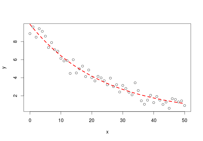
#simulate some data, this without a priori knowledge of the parameter value
y<-runif(1,5,15)*exp(-runif(1,0.01,0.05)*x)+rnorm(51,0,0.5)
#visually estimate some starting parameter values
plot(x,y)
#from this graph set approximate starting values
a_start<-8 #param a is the y value when x=0
b_start<-2*log(2)/a_start #b is the decay rate
#model
m<-nls(y~a*exp(-b*x),start=list(a=a_start,b=b_start))
#get some estimation of goodness of fit
cor(y,predict(m))
#plot the fit
lines(x,predict(m),col="red",lty=2,lwd=3)
[1] 0.9811831
Here it is the plot:
Using SelfStarting function
It is very common for different scientific fields to use different parametrization (i.e. different equations) for the same model, one example is the logistic population growth model, in ecology we use the following form:
$$ N_{t} = \frac{K*N_{0}*e^{r*t}}{K + N_{0} * (e^{r*t} – 1)} $$
With \(N_{t}\) being the number of individuals at time \(t\), \(r\) being the population growth rate and \(K\) the carrying capacity. We can re-write this as a differential equation:
$$ dN/dt = R*N*(1-N/K) $$
library(deSolve)
#simulating some population growth from the logistic equation and estimating the parameters using nls
log_growth <- function(Time, State, Pars) {
  with(as.list(c(State, Pars)), {
    dN <- R*N*(1-N/K)
    return(list(c(dN)))
  })
}
#the parameters for the logisitc growth
pars  <- c(R=0.2,K=1000)
#the initial numbers
N_ini  <- c(N=1)
#the time step to evaluate the ODE
times <- seq(0, 50, by = 1)
#the ODE
out   <- ode(N_ini, times, log_growth, pars)
#add some random variation to it
N_obs<-out[,2]+rnorm(51,0,50)
#numbers cannot go lower than 1
N_obs<-ifelse(N_obs<1,1,N_obs)
#plot
plot(times,N_obs)
This part was just to simulate some data with random error, now come the tricky part to estimate the starting values.
Now R has a built-in function to estimate starting values for the parameter of a logistic equation (SSlogis) but it uses the following equation:
$$ N_{t} = \frac{alpha}{1+e^{\frac{xmid-t}{scale}}} $$
#find the parameters for the equation
SS<-getInitial(N_obs~SSlogis(times,alpha,xmid,scale),data=data.frame(N_obs=N_obs,times=times))
We use the function getInitial which gives some initial guesses about the parameter values based on the data. We pass to this function a selfStarting model (SSlogis) which takes as argument an input vector (the t values where the function will be evaluated), and the un-quoted name of the three parameter for the logistic equation.
However as the SSlogis use a different parametrization we need to use a bit of algebra to go from the estimated self-starting values returned from SSlogis to the one that are in the equation we want to use.
#we used a different parametrization
K_start<-SS["alpha"]
R_start<-1/SS["scale"]
N0_start<-SS["alpha"]/(exp(SS["xmid"]/SS["scale"])+1)
#the formula for the model
log_formula<-formula(N_obs~K*N0*exp(R*times)/(K+N0*(exp(R*times)-1)))
#fit the model
m<-nls(log_formula,start=list(K=K_start,R=R_start,N0=N0_start))
#estimated parameters
summary(m)
#get some estimation of goodness of fit
cor(N_obs,predict(m))
Formula: N_obs ~ K * N0 * exp(R * times)/(K + N0 * (exp(R * times) - 1))

Parameters:
    Estimate Std. Error t value Pr(>|t|)
K  1.012e+03  3.446e+01  29.366   <2e-16 ***
R  2.010e-01  1.504e-02  13.360   <2e-16 ***
N0 9.600e-01  4.582e-01   2.095   0.0415 *
---
Signif. codes:  0 ‘***’ 0.001 ‘**’ 0.01 ‘*’ 0.05 ‘.’ 0.1 ‘ ’ 1

Residual standard error: 49.01 on 48 degrees of freedom

Number of iterations to convergence: 1
Achieved convergence tolerance: 1.537e-06

[1] 0.9910316
Lets plot it:
lines(times,predict(m),col="red",lty=2,lwd=3)
Here it is the plot:
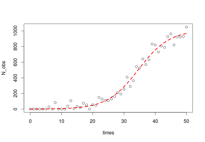
That was a bit of a hassle to get from the SSlogis parametrization to our own, but it was worth it!
In a next post we will see how to go beyond non-linear least square to embrace maximum likelihood estimation methods which are way more powerful and reliable. They allow you to build any model that you can imagine.
why di you write the logistic function with other parameters that the logistic one in R?
This is because in ecology we usually use this formulation: https://en.wikipedia.org/wiki/Logistic_function#In_ecology:_modeling_population_growth, with three parameters: K, the carrying capacity; r, the growth rate and N0 the initial population size. The model / curve is the same, the only different is in the interpretation of the parameters.
why is b_start = 2* log(2)/a_start?
“The best way to get starting values is to eyeball the data…” . I don’t think that’s quite true. My experience is that an evolutionary search, such as the Stochastic Funnel Algorithm, can give VERY good starting values. The SFA, starting from a broad search space, can track down through the SSE to the basin of attraction of the best parameters.
minimizing L2 of the error vector for polynomial models is still linear regression. Readers might want to understand the difference between linear/nonlinear X models/regression, and that you can only get linear regression with L2 of the simple difference error vector.
looking forward for MLE method!
very interesting and clear, thank you.
When will we see the post about maximum likelihood estimation methods?
Thanks for your kind comment! I’ll try to publish the MLE post by mid-march. If you have in mind some specific aspects on this topic that you’d like to hear about, just drop another comment.