In this post we are going to have a look at one of the problems while applying clustering algorithms such as k-means and expectation maximization that is of determining the optimal number of clusters. The problem of determining what will be the best value for the number of clusters is often not very clear from the data set itself. There are a couple of techniques we will walk-through in this post which one can use to help determine the best k-value for a given data set.
To showcase these techniques we will use one of the readily available dataset from the UCI_Dataset_StudentKnowledge.
We will download the dataset in the current R studio environment:
library(readr)
StudentKnowledgeData <- read_csv("YourdownloadFolderPath/StudentKnowledgeData.csv")
View(StudentKnowledgeData)
Pre-processing
This dataset is comma-separated with a header line. We will check for NA values and check if there are any categorical variable to ensure the data is ready for processing for the clustering algorithms. As this data set has low feature vector we will not focus on feature selection aspects but will work with all the available features.
mydata  = StudentKnowledgeData
#let us analyze the data to find if categorical variables are there and if so
#transform them.
mydata = as.data.frame(unclass(mydata))
summary(mydata)
dim(mydata)
# We can now remove any records that have NAs
myDataClean = na.omit(mydata)
dim(myDataClean)
summary(myDataClean)
[1] 402   5
      STG              SCG              STR              LPR
 Min.   :0.0000   Min.   :0.0000   Min.   :0.0100   Min.   :0.0000
 1st Qu.:0.2000   1st Qu.:0.2000   1st Qu.:0.2700   1st Qu.:0.2500
 Median :0.3025   Median :0.3000   Median :0.4450   Median :0.3300
 Mean   :0.3540   Mean   :0.3568   Mean   :0.4588   Mean   :0.4324
 3rd Qu.:0.4800   3rd Qu.:0.5100   3rd Qu.:0.6800   3rd Qu.:0.6500
 Max.   :0.9900   Max.   :0.9000   Max.   :0.9500   Max.   :0.9900
Once we have done pre-processing to ensure the data is ready for further applications. Let us try and scale and center this dataset.
scaled_data = as.matrix(scale(myDataClean))
Clustering Algorithm – k means a sample example of finding optimal number of clusters in it
Let us try to create the clusters for this data. As we can observe this data doesnot have a pre-defined class/output type defined and so it becomes necessary to know what will be an optimal number of clusters.Let us choose random value of cluster numbers for now and see how the clusters are created.
Let us start with k=3 and check what the results are. R comes with a builtin kmeans() function and we do not need to import any extra package for this.
#Let us apply kmeans for k=3 clusters
kmm = kmeans(scaled_data,3,nstart = 50,iter.max = 15) #we keep number of iter.max=15 to ensure the algorithm converges and nstart=50 to #ensure that atleat 50 random sets are choosen
kmm
K-means clustering with 3 clusters of sizes 93, 167, 142

Cluster means:
           STG        SCG        STR        LPR        PEG
1  0.573053974  0.3863411  0.2689915  1.3028712  0.1560779
2 -0.315847301 -0.4009366 -0.3931942 -0.1794893 -0.8332218
3 -0.003855777  0.2184978  0.2862481 -0.6421993  0.8776957

Clustering vector:
  1   2   3   4   5   6   7   8   9  10  11  12  13  14  15  16  17  18  19  20  21
...................................................................................

Within cluster sum of squares by cluster:
[1] 394.5076 524.4177 497.7787
 (between_SS / total_SS =  29.3 %)

Available components:
[1] "cluster"      "centers"      "totss"        "withinss"     "tot.withinss"
[6] "betweenss"    "size"         "iter"         "ifault"
When we check the (between_SS / total_SS) we find it to be low. This ratio actually accounts for the amount of total sum of squares of the data points which is between the clusters. We want to increase this value and as we increase the number of clusters we see it increasing , but we do not want to overfit the data. So we see that with k=401 in this we will have 402 clusters which completely overfits the data. So the idea is to find such a value of k for which the model is not overfitting and at the same time clusters the data as per the actual distribution. Let us now approach how we will solve this problem of finding the best number of clusters.
Elbow Method
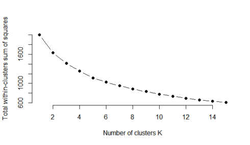
The elbow method looks at the percentage of variance explained as a function of the number of clusters: One should choose a number of clusters so that adding another cluster doesn’t give much better modeling of the data. More precisely, if one plots the percentage of variance explained by the clusters against the number of clusters, the first clusters will add much information (explain a lot of variance), but at some point the marginal gain will drop, giving an angle in the graph. The number of clusters is chosen at this point, hence the “elbow criterion”. This “elbow” cannot always be unambiguously identified.
#Elbow Method for finding the optimal number of clusters
set.seed(123)
# Compute and plot wss for k = 2 to k = 15.
k.max <- 15
data <- scaled_data
wss <- sapply(1:k.max,
              function(k){kmeans(data, k, nstart=50,iter.max = 15 )$tot.withinss})
wss
plot(1:k.max, wss,
     type="b", pch = 19, frame = FALSE,
     xlab="Number of clusters K",
     ylab="Total within-clusters sum of squares")
 [1] 2005.0000 1635.8573 1416.7041 1253.9959 1115.4657 1026.0506  952.4835  887.7202
 [9]  830.8277  780.2121  735.6714  693.7745  657.0939  631.5901  608.3576
Therefore for k=4 the between_ss/total_ss ratio tends to change slowly and remain less changing as compared to other k’s.so for this data k=4 should be a good choice for number of clusters however k=5 also seems to be a potential candidate. So how do we decide what will be the optimal choice. So we look at the second approach which comes with a new package.
Bayesian Inference Criterion for k means
The k-means model is “almost” a Gaussian mixture model and one can construct a likelihood for the Gaussian mixture model and thus also determine information criterion values.
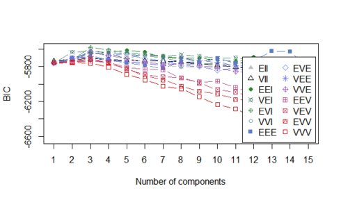
We install the mclust package and we will use the Mclust method of it.Determine the optimal model and number of clusters according to the Bayesian Information Criterion for expectation-maximization, initialized by hierarchical clustering for parameterized Gaussian mixture models. In this method we had set the modelNames parameter to mclust.options(“emModelNames”) so that it includes only those models for evaluation where the number of observation is greater than the dimensions of the dataset here 402>5. The best model selected was EVI (Equal Volume but Variable shape and using Identity Matrix for the eigen values) with number of clusters 3 and 4. So based on this and the previous method the natural number of clusters choice was 4. To further validate this we checked for the BIC(Bayesian Information Criterion for k means) and it seems to validate the findings of Mclust package showing that cluster choice of 3 and 4 are the best and of highest value for this distribution of data.
d_clust <- Mclust(as.matrix(scaled_data), G=1:15,
                  modelNames = mclust.options("emModelNames"))
d_clust$BIC
plot(d_clust)
Bayesian Information Criterion (BIC):
         EII       VII       EEI       VEI       EVI       VVI       EEE       EVE
1  -5735.105 -5735.105 -5759.091 -5759.091 -5759.091 -5759.091 -5758.712 -5758.712
2  -5731.019 -5719.188 -5702.988 -5635.324 -5725.379 -5729.256 -5698.095 -5707.733
3  -5726.577 -5707.840 -5648.033 -5618.274 -5580.305 -5620.816 -5693.977 -5632.555
..................................................................................
         VEE       VVE       EEV       VEV       EVV       VVV
1  -5758.712 -5758.712 -5758.712 -5758.712 -5758.712 -5758.712
2  -5704.051 -5735.383 -5742.110 -5743.216 -5752.709 -5753.597
3  -5682.312 -5642.217 -5736.306 -5703.742 -5717.796 -5760.915
..............................................................

Top 3 models based on the BIC criterion:
    EVI,3     EVI,4     EEI,5
-5580.305 -5607.980 -5613.077
> plot(d_clust)
Model-based clustering plots:

1: BIC
2: classification
3: uncertainty
4: density

Selection: 1
The plot can be seen below where k=3 and k=4 are the best choices available.

As we can see from the two approaches we can to a certain extent be sure of what an optimal value for the number of clusters can be for a clustering problem. There are few other techniques which can also be used. Let us take at one such approach using the NbClust
NbClust package provides 30 indices for determining the number of clusters and proposes to user the best clustering scheme from the different results obtained by varying all combinations of number of clusters, distance measures, and clustering methods
install.packages("NbClust",dependencies = TRUE)
library(NbClust)
nb <- NbClust(scaled_data, diss=NULL, distance = "euclidean",
              min.nc=2, max.nc=5, method = "kmeans",
              index = "all", alphaBeale = 0.1)
hist(nb$Best.nc[1,], breaks = max(na.omit(nb$Best.nc[1,])))
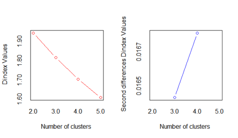
There is an important point to here that this method always takes into the majority of the indexes for each cluster size. So it is important to understand which of the indexes are relevant to the data and based on it to determine if the best choice is the maximum value suggested or any other value.
As we see below looking at the Second differences D-index graph we know it is quite clear the best number of clusters is k=4.
Hope this gives some of the insight how to use different resources in R to determine the optimal number of clusters for relocation algorithms like Kmeans or EM.

