Since the initial publication of the Three Factor Model by Eugene Fama and Kenneth French in their influential 1993 paper (Common Risk Factors in the Returns of Stocks and Bonds) a lot of academic research has been dedicated to the analysis of factors driving security returns. With the rise of quantitative investment management, this field has also attracted increasing awareness of practitioners trying to find factors that help them to select securities that generate superior returns or analyze the driving forces behind realized portfolio returns.
Fortunately, Eugene Fama and Kenneth French still publish the returns of various investment factors analyzed by them on their homepage on a regular basis. While this can be quite handy for academics as well as practitioners, the structure of the Research Library makes accessing these resources a time consuming manual task. The following script, therefore, provides its users with a handy tool that downloads, transforms and visualizes this data.
The user thereby needs to provide the respective CSV file's name as well as a number of rows to skip in the CSV until the portfolio names. Unfortunately, this number differs and therefore needs to be provided individually for each factor. Please examine the structure of the respective CSV files first to provide the correct number of rows to skip otherwise the function will return an error. Setting this up is an annoying manual work at the beginning but, assuming that Eugene Fama and Kenneth French won't change the structure of their CSV sheets, it only needs to be accomplished once. The function then provides a list element, containing the original returns data as well as the indexed returns since start.
The script includes a complete example based on the Three Factor Model.
Compile Function
get_fama_french_data<-function(database,skip_rows)
{
  # The URL for the data.
  ff.url.partial <- paste("http://mba.tuck.dartmouth.edu",
                          "pages/faculty/ken.french/ftp", sep="/")


  #*******************************************************************************#
  #             First download Fama-French three-factor data                      #
  #*******************************************************************************#


  # Download the data and unzip it
  #ff.url <- paste(ff.url.partial, "F-F_Research_Data_Factors_CSV.zip", sep="/")
  #ff.url <- paste(ff.url.partial, "Portfolios_Formed_on_OP_CSV.zip", sep="/")
  ff.url <- paste(ff.url.partial, database, sep="/")

  # get the file url
  today = as.Date(Sys.time())
  forecasturl = ff.url
  # create a temporary directory
  td = tempdir()
  # create the placeholder file
  tf = tempfile(tmpdir=td, fileext=".zip")
  # download into the placeholder file
  download.file(forecasturl, tf)

  #*******************************************************************************#
  #                     Second Unzip File and Create a data.frame                 #
  #*******************************************************************************#
  # get the name of the first file in the zip archive
  fname = unzip(tf, list=TRUE)$Name[1]
  # unzip the file to the temporary directory
  unzip(tf, files=fname, exdir=td, overwrite=TRUE)
  # fpath is the full path to the extracted file
  fpath = file.path(td, fname)

  # stringsAsFactors=TRUE will screw up conversion to numeric!
  #skip_rows<-18
  d = read.csv(fpath, header=T, row.names=NULL,
               stringsAsFactors=F, skip=skip_rows)

  #
  d<-d[!is.na(d$X),]


  #*******************************************************************************#
  #                     Third Calculate Indexed Portfolio Returns                 #
  #*******************************************************************************#
  indexed_ret<-function(x)
  {
    x<-as.numeric(x)
    x<-cumprod(1+(x/100))
    return(x)
  }

  indexed_ret<-as.data.frame(apply(subset(d,select=c(-X)),2,indexed_ret))

  d$date<-as.Date(paste(substr(d$X,1,4),"-",substr(d$X,5,6),"-01",sep=""))
  indexed_ret$date<-d$date

  indexed_ret<-indexed_ret[!is.na(indexed_ret[,1]),]
  d<-head(d,nrow(indexed_ret))

  #*******************************************************************************#
  #                         Fourth Combine to List Element                        #
  #*******************************************************************************#
  factor_ret<-list(d=d,indexed_ret=indexed_ret)
}
#-----------------------------------------------------------------------------------------------------------------------
Retrieve Data
three_factor_model<-get_fama_french_data("F-F_Research_Data_Factors_CSV.zip",3)
## Error in download.file(forecasturl, tf): cannot open URL 'http://mba.tuck.dartmouth.edu/pages/faculty/ken.french/ftp/F-F_Research_Data_Factors_CSV.zip'
Examine Returns Data
head(three_factor_model$d,5)
##        X   Mkt.RF      SMB      HML       RF       date
## 1 192607     2.96    -2.30    -2.87     0.22 1926-07-01
## 2 192608     2.64    -1.40     4.19     0.25 1926-08-01
## 3 192609     0.36    -1.32     0.01     0.23 1926-09-01
## 4 192610    -3.24     0.04     0.51     0.32 1926-10-01
## 5 192611     2.53    -0.20    -0.35     0.31 1926-11-01
Examine Indexed Returns Data
head(three_factor_model$indexed_ret,5)
##     Mkt.RF       SMB      HML       RF       date
## 1 1.029600 0.9770000 0.971300 1.002200 1926-07-01
## 2 1.056781 0.9633220 1.011997 1.004706 1926-08-01
## 3 1.060586 0.9506061 1.012099 1.007016 1926-09-01
## 4 1.026223 0.9509864 1.017260 1.010239 1926-10-01
## 5 1.052186 0.9490844 1.013700 1.013371 1926-11-01
Plot Indexed Portfolio Returns with Plotly
This is just included as an example. Unfortunately Plotly Charts don't seem to get rendered very nicely on DataScience+. I am therefore providing another example with my own base-R plot function given below
#
#Fama French 3 Factor Model
#plot_ly(three_factor_model$indexed_ret,x=~date,y=~SMB,name="Size",type="scatter",mode="line")%>%
#  add_trace(three_factor_model$indexed_ret,x=~date,y=~HML,name="Value")%>%
#  add_trace(three_factor_model$indexed_ret,x=~date,y=~RF,name="Risk-Free")%>%
#  layout(title="3 Factor Model",xaxis = list(title=""), yaxis = list(title=""),legend = list(orientation = "h",xanchor = "center",x = 0.5))
Design Function
This function takes care of the chart's layout.
#First Axis
chart_design<-function(y_min,y_max,x_min,x_max,y_caption,titel,x_freq)
{
  options(warn=-1)
  par(mfrow=c(1,1))      # number of rows, number of columns
  par(bg = "transparent")
  #op <- par(mar = c(4,4,4,4) + 0.8)

  plot(as.Date(df$date),df$value,
       main=titel,                     # Chart Titel
       xlab="",                         # x-Achsenbeschriftung
       ylab=y_caption,                     # y-Achsenbeschriftung
       type="l",                        # type
       col=col1,                        # farbe
       xlim=c(x_min, x_max),
       ylim=c(y_min,y_max),                # y-achse
       lwd = 2,                         # thickness of the line
       bty = "n",                       # Remove the box around the plot
       font.axis = 2,                   # Change axis font to bold italic
       col.axis = "black",              # Set the color of the axis
       las=1,                            # Make axis labels parallel to x-axis (2 for vertical)
       xaxt='n',                       # Delete x-axis
       font.main=10,
       cex.main=1.1,
       cex.lab=1.1,
       font.lab=6,
       font.axis=6,
       cex.axis=1.1,
       tck=-0.01,
       col.axis="black",
       col.ticks="grey"
  )
  grid(NA,NULL,lwd=1.5,col = 'grey')

  abline(h = 0,
         col = 'grey', lty = "solid",lwd=1.5)

  abline(v=axis.Date(1,font.axis=6,tck=-0.01,cex.axis=1.1,col.ticks="grey",font.lab=6,lwd=1.3, at=seq(as.Date(x_min), x_max, by=x_freq), format="%m-%Y"),
         col = 'grey', lty = "dotted",lwd=1.5)

  lines(as.Date(df$date),df$value,col=col1,lwd=2)

  box(bty = "l")
  options(warn=0)
  #****
}
Annotate Last Value in Time Series
This function enables the user to add a caption to the last point in the plotted time-series.
last_value_function_a<-function(datum,zeitreihe,function_color,position_a)
{
  names(df)[names(df)==datum]<-"function_tmp_date"
  names(df)[names(df)==zeitreihe]<-"function_tmp_value"

  wert<-tail(df$function_tmp_value[!is.na(df$function_tmp_value)],1)
  round_wert<-round(wert,digits=2)
  datum_last<-as.Date(tail(df$function_tmp_date[!is.na(df$function_tmp_date)],1))
  text(datum_last, wert,paste(round_wert,sep=""),col=function_color,font =6,pos = position_a)

  names(df)[names(df)=="function_tmp_date"]<-datum
  names(df)[names(df)=="function_tmp_value"]<-zeitreihe

}
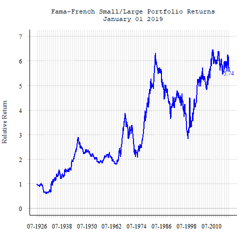
Plot Indexed Portfolio Returns Custom Function
df<-three_factor_model$indexed_ret
names(df)[names(df)=="SMB"]<-"value"

col1<-"blue"
chart_design(
  y_min=min(pretty(extendrange(df$value))),
  y_max=max(pretty(extendrange(df$value))),
  x_min=min(df$date),
  x_max=max(df$date),
  y_caption="Relative Return",
  titel=c("Fama-French Small/Large Portfolio Returns",format(max(df$date),"%B %d %Y")),
  x_freq="12 mon"
)
last_value_function_a("date","value","blue",1)