Decision trees are a highly useful visual aid in analyzing a series of predicted outcomes for a particular model. As such, it is often used as a supplement (or even alternative to) regression analysis in determining how a series of explanatory variables will impact the dependent variable.
In this particular example, we analyse the impact of explanatory variables of age, gender, miles, debt, and income on the dependent variable car sales.
Classification Problems and Decision Trees
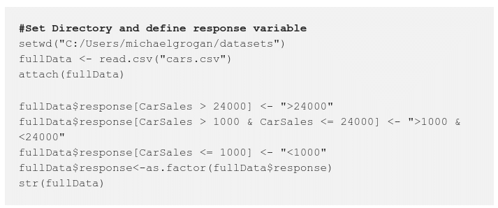
Firstly, we load our dataset and create a response variable (which is used for the classification tree since we need to convert sales from a numerical to categorical variable):
We then create the training and test data (i.e. the data that we will use to create our model and then the data we will test this data against):
#Create training and test data
inputData <- fullData[1:770, ] # training data
testData <- fullData[771:963, ] # test data
Then, our classification tree is created:
#Classification Tree
library(rpart)
formula=response~Age+Gender+Miles+Debt+Income
dtree=rpart(formula,data=inputData,method="class",control=rpart.control(minsplit=30,cp=0.001))
plot(dtree)
text(dtree)
summary(dtree)
printcp(dtree)
plotcp(dtree)
printcp(dtree)
Note that the cp value is what indicates our desired tree size – we see that our X-val relative error is minimized when our size of tree value is 4. Therefore, the decision tree is created using the dtree variable by taking into account this variable.
summary(dtree)
Call:
rpart(formula = formula, data = inputData, method = "class",
    control = rpart.control(minsplit = 30, cp = 0.001))
  n= 770

           CP nsplit
1 0.496598639      0
2 0.013605442      1
3 0.008503401      6
4 0.001000000     10
  rel error    xerror
1 1.0000000 1.0000000
2 0.5034014 0.5170068
3 0.4353741 0.5646259
4 0.4013605 0.5442177
        xstd
1 0.07418908
2 0.05630200
3 0.05854027
4 0.05759793
Tree Pruning
The decision tree is then “pruned”, where inappropriate nodes are removed from the tree to prevent overfitting of the data:
#Prune the Tree and Plot
pdtree<- prune(dtree, cp=dtree$cptable[which.min(dtree$cptable[,"xerror"]),"CP"])
plot(pdtree, uniform=TRUE,
     main="Pruned Classification Tree For Sales")
text(pdtree, use.n=TRUE, all=TRUE, cex=.8)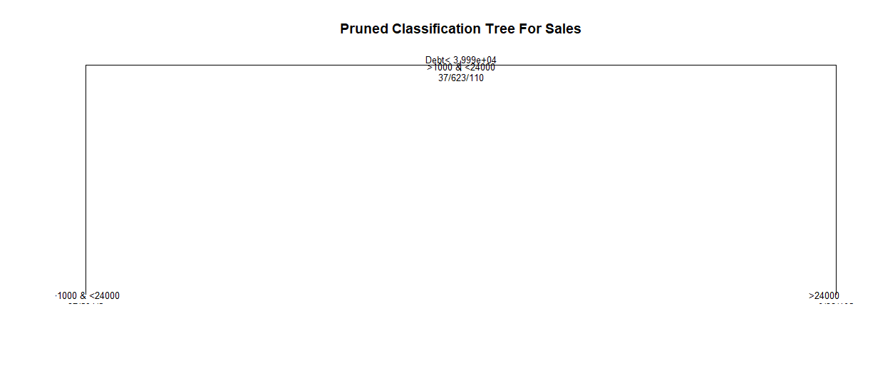
The model is now tested against the test data, and we see that we have a misclassification percentage of 16.75%. Clearly, the lower the better, since this indicates our model is more accurate at predicting the “real” data:
#Model Testing
out
table(out[1:193],testData$response)
response_predicted
response_input
mean(response_input != response_predicted) # misclassification %
[1] 0.2844156
Solving Regression Problems With Decision Trees
When the dependent variable is numerical rather than categorical, we will want to set up a regression tree instead as follows:
#Regression Tree
fitreg <- rpart(CarSales~Age+Gender+Miles+Debt+Income,
method="anova", data=inputData)
printcp(fitreg)
plotcp(fitreg)
summary(fitreg)
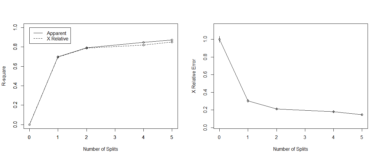
par(mfrow=c(1,2))
rsq.rpart(fitreg) # cross-validation results 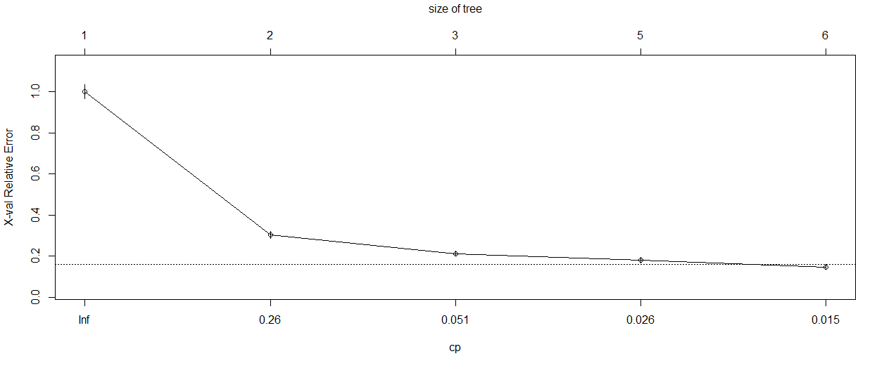
#Regression Tree
fitreg
printcp(fitreg)
Regression tree:
rpart(formula = CarSales ~ Age + Gender + Miles + Debt + Income,
    data = inputData, method = "anova")

Variables actually used in tree construction:
[1] Age    Debt   Income

Root node error: 6.283e+10/770 = 81597576

n= 770

        CP nsplit rel error
1 0.698021      0   1.00000
2 0.094038      1   0.30198
3 0.028161      2   0.20794
4 0.023332      4   0.15162
5 0.010000      5   0.12829
   xerror     xstd
1 1.00162 0.033055
2 0.30373 0.016490
3 0.21261 0.012890
4 0.18149 0.013298
5 0.14781 0.013068
plotcp(fitreg)
summary(fitreg)
Call:
rpart(formula = CarSales ~ Age + Gender + Miles + Debt + Income,
    data = inputData, method = "anova")
  n= 770

          CP nsplit rel error
1 0.69802077      0 1.0000000
2 0.09403824      1 0.3019792
3 0.02816107      2 0.2079410
4 0.02333197      4 0.1516189
5 0.01000000      5 0.1282869
     xerror       xstd
1 1.0016159 0.03305536
2 0.3037301 0.01649002
3 0.2126110 0.01289041
4 0.1814939 0.01329778
5 0.1478078 0.01306756

Variable importance
  Debt  Miles Income    Age
    53     23     20      4
Now, we prune our regression tree:
#Prune the Tree
pfitreg<- prune(fitreg, cp=fitreg$cptable[which.min(fitreg$cptable[,"xerror"]),"CP"]) # from cptable
plot(pfitreg, uniform=TRUE,
     main="Pruned Regression Tree for Sales")
text(pfitreg, use.n=TRUE, all=TRUE, cex=.8)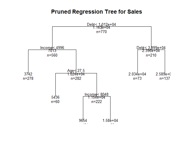
Random Forests
However, what if we have many decision trees that we wish to fit without preventing overfitting? A solution to this is to use a random forest.
A random forest allows us to determine the most important predictors across the explanatory variables by generating many decision trees and then ranking the variables by importance.
library(randomForest)
fitregforest
print(fitregforest) # view results
Call:
 randomForest(formula = CarSales ~ Age + Gender + Miles + Debt +      Income, data = inputData)
               Type of random forest: regression
                     Number of trees: 500
No. of variables tried at each split: 1

          Mean of squared residuals: 10341022
                    % Var explained: 87.33
> importance(fitregforest) # importance of each predictor
       IncNodePurity
Age       5920357954
Gender     187391341
Miles    10811341575
Debt     21813952812
Income   12694331712
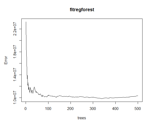
From the above, we see that debt is ranked as the most important factor, i.e. customers with high debt levels will be more likely to spend a greater amount on a car. We see that 87.33% of the variation is “explained” by our random forest, and our error is minimized at roughly 100 trees.