Bayesian regression with STAN: Part 1 normal regression

This post will introduce you to bayesian regression in R, see the reference list at the end of the post for further information concerning this very broad topic.

Bayesian regression

Bayesian statistics turn around the Bayes theorem, which in a regression context is the following: $$ P(\theta|Data) \propto P(Data|\theta) \times P(\theta) $$ Where \(\theta\) is a set of parameters to be estimated from the data like the slopes and Data is the dataset at hand. \(P(\theta)\) is our prior, the knowledge that we have concerning the values that \(\theta\) can take, \(P(Data|\theta)\) is the likelihood and \(P(\theta|Data)\) is the posterior distribution. This equation basically takes our prior knowledge about the parameters (ie do I expect my regression coefficient to be positive or negative), and update this prior knowledge with the likelihood to observe the data for particular parameter values and gives the posterior probability. The posterior probability is the probability of a given parameter value given the data and our prior knowledge. In frequentist statistics the likelihood is the metric under study, in most of the cases however we are not interested in the probability of the data knowing a specific parameter values, but rather to answer statement like: What is the probability that my slope is positive? What is the probability that parameter \(\theta_{1}\) is bigger than parameter \(\theta_{2}\)? Computing the posterior probability using bayesian regression gives direct answers to these types of questions.

Ways to do Bayesian regression in R

There are several packages for doing bayesian regression in R, the oldest one (the one with the highest number of references and examples) is R2WinBUGS using WinBUGS to fit models to data, later on JAGS came in which uses similar algorithm as WinBUGS but allowing greater freedom for extension written by users. Recently STAN came along with its R package: rstan, STAN uses a different algorithm than WinBUGS and JAGS that is designed to be more powerful so in some cases WinBUGS will failed while STAN will give you meaningful answers. Also STAN is faster in execution times.

Example

Let’s see how to do a regression analysis in STAN using a simulated example.
First you need to write a model, don’t worry there are extensive resources online and a user mailing list to guide you on how to write such models. Below is a simple normal regression model:

/*
*Simple normal regression example
*/

data {
  int N; //the number of observations
  int N2; //the size of the new_X matrix
  int K; //the number of columns in the model matrix
  real y[N]; //the response
  matrix[N,K] X; //the model matrix
  matrix[N2,K] new_X; //the matrix for the predicted values
}
parameters {
  vector[K] beta; //the regression parameters
  real sigma; //the standard deviation
}
transformed parameters {
  vector[N] linpred;
  linpred <- X*beta;
}
model {  
  beta[1] ~ cauchy(0,10); //prior for the intercept following Gelman 2008

  for(i in 2:K)
   beta[i] ~ cauchy(0,2.5);//prior for the slopes following Gelman 2008
  
  y ~ normal(linpred,sigma);
}
generated quantities {
  vector[N2] y_pred;
  y_pred <- new_X*beta; //the y values predicted by the model
}

The best way to go is to save this into a .stan file, ie open any text editor, copy/paste the model code and save it as .stan.
A little note concerning the priors, how to set priors in bayesian regression is a big topic and if you are interested you may read this book chapter. Here I used weakly informative priors as defined in Gelman 2008. The idea behind this prior is that most of the effects (slopes) are small and a few are big, therefore the cauchy distribution with mean 0 and a long tail.
We now turn into R, loading the necessary libraries and simulating some data:

#load libraries
library(rstan)
library(coda)
set.seed(20151204)
#the explanatory variables
dat<-data.frame(x1=runif(100,-2,2),x2=runif(100,-2,2))
#the model
X<-model.matrix(~x1*x2,dat)
#the regression slopes
betas<-runif(4,-1,1)
#the standard deviation for the simulated data
sigma<-1
#the simulated data
y_norm<-rnorm(100,X%*%betas,sigma)
#a matrix to get the predicted y values
new_X<-model.matrix(~x1*x2,expand.grid(x1=seq(min(dat$x1),max(dat$x1),length=20),x2=c(min(dat$x2),mean(dat$x2),max(dat$x2))))

In this example I simulated two explanatory variables (x1 and x2) which interact with each other to affect the response variable y, with values that are normally distributed around the expected values. I also created a new_X matrix that will be used to draw the regression lines as predicted by the model. It contains x1 values ordered from the smallest to biggest values as well as three specific x2 values, namely the minimum, mean and maximum value. This is necessary since x1 and x2 interact, we need to draw the regression lines predicted form the models at different values of x2.

Next we fit the model to the data:

#the location of the model files
setwd("/home/lionel/Desktop/Blog/STAN/")
#the model
m_norm<-stan(file="normal_regression.stan",data = list(N=100,N2=60,K=4,y=y_norm,X=X,new_X=new_X),pars = c("beta","sigma","y_pred"))

The stan function take the model file and the data in a list, here you should be careful to match every single variables defined in the data section in the model file. The pars argument is used to specify which parameters to return.
STAN is in constant development, at the time of writing of this post with rstan version 2.8.2 I got a couple of warning that scale parameters are 0. Careful reading of the warning message reveal that there is nothing to worry about with my model. I therefore go one and plot some diagnostics plot.

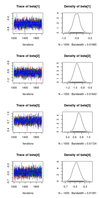
Traceplot and posterior distribution

#plotting the posterior distribution for the parameters
post_beta<-As.mcmc.list(m_norm,pars="beta")
plot(post_beta)

Here it is the plot:

This plot show the traces of the parameters on the left, each color represent a different chain, we had 4 chains (the default) and you want all chain to converge to similar values (ie no divergence in the values on the right side of the plot). On the right side of the plot are the posterior distributions of the parameters, this is the key information one wants to get from a bayesian regression analysis, from these distribution we can ask very important question like: what is the probability that my parameters have a value bigger than 0.

#computing the posterior probability for the slopes to be bigger than 0
apply(extract(m_norm,pars="beta")$beta,2,function(x) length(which(x>0))/4000)
[1] 0 0 1 0

This was easy, parameter beta[3] (slope between y_norm and x2) as a posterior probability of 1 to be bigger than 0 while all the other parameters have a posterior probability of 0 to be bigger than 0.

Pairwise correlation

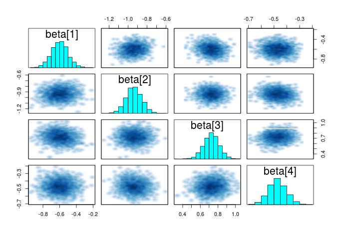
Another helpful summary plot is the pairwise correlation between the parameters, if each parameters is adding additional independent information, the points should form a shapeless cloud. If you have strong correlation between several parameters, then you may consider dropping some as they do not add extra information.

#plot the correlation between the parameters
pairs(m_norm,pars="beta")

Here it is the plot:

Credible intervals around the parameters

Credible intervals are another summary for the different parameters in the models, the red bands in this graph show that the parameters have a probability of 0.8 to be within the bands. Which is an easier summary than the classical frequentist confidence intervals which tells us: “If I repeat my experiment many times, the values of my parameters will be within this interval 80% of the time”.

#plotting credible intervals for the different betas
plot(m_norm,pars=c("beta","sigma"))

Here it is the plot:

Regression line

And finally we plot the regression lines with their credible intervals at different x2 values.

#getting regression curves plus 95% credible intervals
new_x<-data.frame(x1=new_X[,2],x2=rep(c("Min","Mean","Max"),each=20))
new_y<-extract(m_norm,pars="y_pred")
pred<-apply(new_y[[1]],2,quantile,probs=c(0.025,0.5,0.975)) #the median line with 95% credible intervals
#plot
plot(dat$x1,y_norm,pch=16)
lines(new_x$x1[1:20],pred[2,1:20],col="red",lwd=3)
lines(new_x$x1[1:20],pred[2,21:40],col="orange",lwd=3)
lines(new_x$x1[1:20],pred[2,41:60],col="blue",lwd=3)
lines(new_x$x1[1:20],pred[1,1:20],col="red",lwd=1,lty=2)
lines(new_x$x1[1:20],pred[1,21:40],col="orange",lwd=1,lty=2)
lines(new_x$x1[1:20],pred[1,41:60],col="blue",lwd=1,lty=2)
lines(new_x$x1[1:20],pred[3,1:20],col="red",lwd=1,lty=2)
lines(new_x$x1[1:20],pred[3,21:40],col="orange",lwd=1,lty=2)
lines(new_x$x1[1:20],pred[3,41:60],col="blue",lwd=1,lty=2)
legend("topright",legend=c("Min","Mean","Max"),lty=1,col=c("red","orange","blue"),bty = "n",title = "Effect of x2 value on\nthe regression")

Here it is the plot:

We see that for low x2 values, y stay almost constant across the x1 gradient, while as x2 values becomes biggers, the relationship between y and x1 become more negatives (steeper declining curves).

Summary

In this post we saw how to fit normal regression using STAN and how to get a set of important summaries from the models. The STAN model presented here should be rather flexible and could be fitted to dataset of varying sizes. Remember that the explanatory variables should be standardized before fitting the models. This is just a first glimpse into the many models that can fitted using STAN, in a later posts we will look at generalized linear models, extending to non-normal models with various link functions and also to hierarchical models.

References

The bible in Bayesian analysis; Applied textbook focused for ecologist; The STAN reference guide; A book to rethink stats