This is a pretty short post on an issue that popped at some point in the past, at that time I found a way around it but as it arose again recently I decided to go through it.
The issue I had was that when modeling an interaction between a continuous (say temperature) and a categorical variables (say site ID), we get the slope for the first level (the baseline) of the categorical variable and the difference between the remaining levels and this baseline slope. Sometime it is not only interesting to get if we have differences between the levels but also to know if the slopes at the different levels are different from 0.
Let’s see how this works:
set.seed(20160315)
#simulate some data
X<-data.frame(Temp=runif(100,-2,2),Site=gl(n=2,k=50))
#the model matrix
mm<-model.matrix(~Temp*Site,X)
#the coefficients for the models
bs<-c(1,1.5,-2,3)
#simulate the response
X$y<-rnorm(100,mean=mm%*%bs,sd=1)
#fit the model
m<-lm(y~Temp*Site,X)
#summary table
summary(m)
Call:
lm(formula = y ~ Temp * Site, data = X)

Residuals:
    Min      1Q  Median      3Q     Max
-2.2194 -0.6776 -0.1545  0.5517  2.7618

Coefficients:
            Estimate Std. Error t value Pr(>|t|)
(Intercept)   0.9904     0.1474   6.717 1.31e-09 ***
Temp          1.6274     0.1280  12.715  < 2e-16 ***
Site2        -1.9410     0.2083  -9.319 4.33e-15 ***
Temp:Site2    3.0109     0.1842  16.343  < 2e-16 ***
---
Signif. codes:  0 ‘***’ 0.001 ‘**’ 0.01 ‘*’ 0.05 ‘.’ 0.1 ‘ ’ 1

Residual standard error: 1.031 on 96 degrees of freedom
Multiple R-squared:  0.943,	Adjusted R-squared:  0.9412
F-statistic: 528.9 on 3 and 96 DF,  p-value: < 2.2e-16
The code below is for making a plot:
#a nice plot
new_x<-seq(-2,2,length=10)
plot(y~Temp,X,col=c("red","blue")[X$Site],pch=16)
lines(new_x,coef(m)["(Intercept)"]+coef(m)["Temp"]*new_x,col="red",lwd=3)
lines(new_x,(coef(m)["(Intercept)"]+coef(m)["Site2"])+(coef(m)["Temp"]+coef(m)["Temp:Site2"])*new_x,col="blue",lwd=3)
Here is the plot:
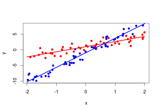
From the summary table of this model we see that the slopes between y and Temp is significantly bigger in Site 2 compared to Site 1. But this does not tell us if the slope y~Temp is different from 0 in Site 2.
Getting the slope y~Temp in Site 2 is easy:
#get the estimated slope for Site2
b<-coef(m)[2]+coef(m)[4]
But we need some estimation of uncertainty (ie standard error) around this slope to get to a p-value. We can achieve this by knowing that:
Var(a+b) = Var(a) + Var(b) + 2*cov(a,b)
It is rather easy to get this information from a lm object in R, the vcov function return the variance-covariance matrix of the model coefficient. The diagonal values are the coefficient variances and the off-diagonal values are the covariances. The standard error is then the square root of the variance.
#get the standard error for the slope of Site2
se<-sqrt(vcov(m)["Temp","Temp"]+vcov(m)["Temp:Site2","Temp:Site2"]+2*vcov(m)["Temp","Temp:Site2"])
#compute the two-sided p-values that the slope for Fac2 is different from 0
pt(b/se, df = nrow(X)-length(coef(m)),lower.tail=FALSE)*2
You can of course extend this to more than two-way interactions and for categorical variables with more than two levels. You just need to be careful when computing the different slopes and standard errors that you took all the appropriate coefficients.
Of course you may also fit separate models for each levels of your categorical variables, you should find the same results. The nice thing about fitting one model is that you get some indication about differences between the different levels which you would not get so easily from separate models …


Also, I think you may have accidentally posted an old example of your code; while the model part at the beginning uses variables ‘Site’ and ‘Temp’, the rest (plotting and getting stuff out of the model) uses ‘Fac’ and ‘x’, which causes the code to crash; also, the code for the plot doesn’t add the scatter points.
Here’s the code that would recreate our example, as best as I could backwards-engineer it:
set.seed(20160315)
#simulate some data
X<-data.frame(Temp=runif(100,-2,2),Site=gl(n=2,k=50))
#the model matrix
mm<-model.matrix(~Temp*Site,X)
#the coefficients for the models
bs<-c(1,1.5,-2,3)
#simulate the response
X$y<-rnorm(100,mean=mm%*%bs,sd=1)
#fit the model
m<-lm(y~Temp*Site,X)
#summary table
summary(m)
#a nice plot
new_x<-seq(-2,2,length=10)
plot(y~Temp,X,col=c("red","blue")[X$Fac],pch=16)
lines(new_x,coef(m)["(Intercept)"]+coef(m)["Temp"]*new_x,col="red",lwd=3)
lines(new_x,(coef(m)["(Intercept)"]+coef(m)["Site2"])+(coef(m)["Temp"]+coef(m)["Temp:Site2"])*new_x,col="blue",lwd=3)
points( X[X$Site==1,"Temp"], X[X$Site==1,"y"], col="red", pch=19 )
points( X[X$Site==2,"Temp"], X[X$Site==2,"y"], col="blue", pch=19 )
#get the estimated slope for Fac2
b<-coef(m)[2]+coef(m)[4]
#get the standard error for the slope of Fac2
se<-sqrt(vcov(m)["Temp","Temp"]+vcov(m)["Temp:Site2","Temp:Site2"]+2*vcov(m)["Temp","Temp:Site2"])
#compute the two-sided p-values that the slope for Fac2 is different from 0
pt(b/se, df = nrow(X)-length(coef(m)),lower.tail=FALSE)*2
Thanks for getting this! Copy/pasting is the worst enemy of blogger …
An even easier way to do this is to nest the factors:
m<-lm(y~Site/Temp,X)
This model gives the slope for each level of Site. And while the coefficients are expressed in the same way, it's essentially the same model (you can check both the nested and crossed models to see that they have the same R2, etc.); it's the same idea as using e.g. dummy vs. sum vs. helmert coding, which will give coefficients representing different things but still ultimately have the same fit.
Cool Stuff! Used similar nested formula in mixed-effect models ie (1|Site/Plot) for plots nested within sites, never used it beyond this so far. So thanks for sharing this!
Thanks this is very useful information. Yet another way is the re-parametrisation below
1. Calculate X1 = X * Z (i.e = exposure condition is met, zero otherwise).
2. Calculate X0 = X * (1-Z) (i.e. = exposure for NON-condition, zero otherwise).
3. Instead of X, Z and XZ, fit X1, X0 and Z.
“`r
X$Site1_Temp <- X$Temp * (X$Site == '1')
X$Site2_Temp <- X$Temp * (X$Site == '2')
m3 <- lm(y ~ Site + Site1_Temp + Site2_Temp, data = X)
summary(m3)
# in addition this allows to explore complex responses like curves using GAMs
library(mgcv)
# let's make this response function more interesting
X$y2 <- ifelse(X$Site == 1, X$y + X$Temp^2, X$y)
# mgcv uses GCV and penalised splines to estimate best curve
m3.1 <- gam(y2 ~ Site + s(Site1_Temp) + Site2_Temp, data = X)
summary(m3.1)
# and easily plot the partial residuals
png("interactions_with_gam_example.png")
par(mfrow = c(2,1))
plot(m3.1, select = 1, se = T)
plot(m3.1, select = 3, se = T, all.terms = T)
dev.off()
“`
This model also contains three parameters and captures the same interactions as it is the same model with a different parametrisation. The standard errors for the X1 and X0 coefficients are available directly from the regression output.
I find this method easier to interpret and is considerably more flexible than the other two approaches when many interaction terms are being compared. A limitation remains for this method in that the pre-processing steps required are more complicated, and there are inherently more possibilities for the data analyst to make errors in writing their code as they make these changes to the analytical data.