t-SNE is a very powerful technique that can be used for visualising (looking for patterns) in multi-dimensional data. Great things have been said about this technique. In this blog post I did a few experiments with t-SNE in R to learn about this technique and its uses.
Its power to visualise complex multi-dimensional data is apparent, as well as its ability to cluster data in an unsupervised way.
What’s more, it is also quite clear that t-SNE can aid machine learning algorithms when it comes to prediction and classification. But the inclusion of t-SNE in machine learning algorithms and ensembles has to be ‘crafted’ carefully, since t-SNE was not originally intended for this purpose.
All in all, t-SNE is a powerful technique that merits due attention.
t-SNE
Let’s start with a brief description. t-SNE stands for t-Distributed Stochastic Neighbor Embedding and its main aim is that of dimensionality reduction, i.e., given some complex dataset with many many dimensions, t-SNE projects this data into a 2D (or 3D) representation while preserving the ‘structure’ (patterns) in the original dataset. Visualising high-dimensional data in this way allows us to look for patterns in the dataset.
t-SNE has become so popular because:
- it was demonstrated to be useful in many situations,
- it’s incredibly flexible, and
- can often find structure where other dimensionality-reduction algorithms cannot.
A good introduction on t-SNE can be found here. The original paper on t-SNE and some visualisations can be found at this site. In particular, I like this site which shows how t-SNE is used for unsupervised image clustering.
While t-SNE itself is computationally heavy, a faster version exists that uses what is known as the Barnes-Hut approximation. This faster version allows t-SNE to be applied on large real-world datasets.
t-SNE for Exploratory Data Analysis
Because t-SNE is able to provide a 2D or 3D visual representation of high-dimensional data that preserves the original structure, we can use it during initial data exploration. We can use it to check for the presence of clusters in the data and as a visual check to see if there is some ‘order’ or some ‘pattern’ in the dataset. It can aid our intuition about what we think we know about the domain we are working in.
Apart from the initial exploratory stage, visualising information via t-SNE (or any other algorithm) is vital throughout the entire analysis process – from those first investigations of the raw data, during data preparation, as well as when interpreting the outputs of machine learning algorithms and presenting insights to others. We will see further on that we can use t-SNE even during the predcition/classification stage itself.
Experiments on the Optdigits dataset
In this post, I will apply t-SNE to a well-known dataset, called optdigits, for visualisation purposes.
The optdigits dataset has 64 dimensions. Can t-SNE reduce these 64 dimensions to just 2 dimension while preserving structure in the process? And will this structure (if present) allow handwritten digits to be correctly clustered together? Let’s find out.
tsne package
We will use the tsne package that provides an exact implementation of t-SNE (not the Barnes-Hut approximation). And we will use this method to reduce dimensionality of the optdigits data to 2 dimensions. Thus, the final output of t-SNE will essentially be an array of 2D coordinates, one per row (image). And we can then plot these coordinates to get the final 2D map (visualisation). The algorithm runs in iterations (called epochs), until the system converges. Every
\(K\) number of iterations and upon convergence, t-SNE can call a user-supplied callback function, and passes the list of 2D coordinates to it. In our callback function, we plot the 2D points (one per image) and the corresponding class labels, and colour-code everything by the class labels.
traindata <- read.table("optdigits.tra", sep=",")
trn <- data.matrix(traindata)

require(tsne)

cols <- rainbow(10)

# this is the epoch callback function used by tsne.
# x is an NxK table where N is the number of data rows passed to tsne, and K is the dimension of the map.
# Here, K is 2, since we use tsne to map the rows to a 2D representation (map).
ecb = function(x, y){ plot(x, t='n'); text(x, labels=trn[,65], col=cols[trn[,65] +1]); }

tsne_res = tsne(trn[,1:64], epoch_callback = ecb, perplexity=50, epoch=50)
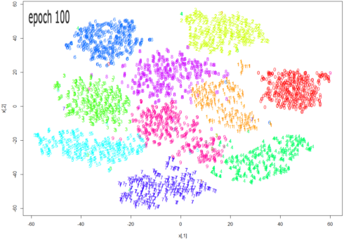
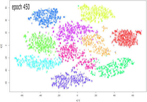
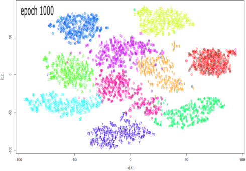
The images below show how the clustering improves as more epochs pass.
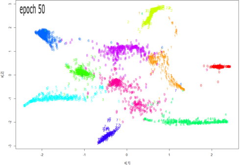
As one can see from the above diagrams (especially the last one, for epoch 1000), t-SNE does a very good job in clustering the handwritten digits correctly.
But the algorithm takes some time to run. Let’s try out the more efficient Barnes-Hut version of t-SNE, and see if we get equally good results.
Rtsne package
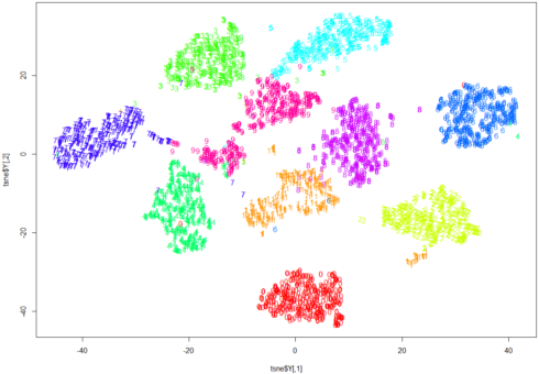
The Rtsne package can be used as shown below. The perplexity parameter is crucial for t-SNE to work correctly – this parameter determines how the local and global aspects of the data are balanced. A more detailed explanation on this parameter and other aspects of t-SNE can be found in this article, but a perplexity value between 30 and 50 is recommended.
traindata <- read.table("optdigits.tra", sep=",")
trn <- data.matrix(traindata)

require(Rtsne)

# perform dimensionality redcution from 64D to 2D
tsne <- Rtsne(as.matrix(trn[,1:64]), check_duplicates = FALSE, pca = FALSE, perplexity=30, theta=0.5, dims=2)

# display the results of t-SNE
cols <- rainbow(10)
plot(tsne$Y, t='n')
text(tsne$Y, labels=trn[,65], col=cols[trn[,65] +1])
Note how clearly-defined and distinctly separable the clusters of handwritten digits are. We have only a minimal amount of incorrect entries in the 2D map.
Of Manifolds and the Manifold Assumption
How can t-SNE achieve such a good result? How can it ‘drop’ 64-dimensional data into just 2 dimensions and still preserve enough (or all) structure to allow the classes to be separated?
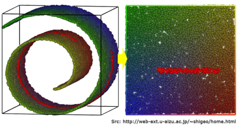
The reason has to do with the mathematical concept of manifolds. A Manifold is a \(d\)-dimensional surface that lives in an \(D\)-dimensional space, where \(d < D\). For the 3D case, imagine a 2D piece of paper that is embedded within 3D space. Even if the piece of paper is crumpled up extensively, it can still be ‘unwrapped’ (uncrumpled) into the 2D plane that it is. This 2D piece of paper is a manifold in 3D space. Or think of an entangled string in 3D space – this is a 1D manifold in 3D space.
Now there’s what is known as the Manifold Hypothesis, or the >Manifold Assumption, that states that natural data (like images, etc.) forms lower dimensional manifolds in their embedding space. If this assumption holds (there are theoretical and experimental evidence for this hypothesis), then t-SNE should be able to find this lower-dimensional manifold, ‘unwrap it’, and present it to us as a lower-dimensional map of the original data.
t-SNE vs. SOM
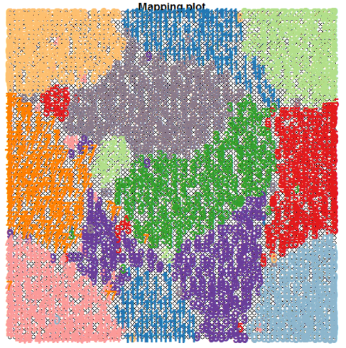
t-SNE is actually a tool that does something similar to Self-Organising Maps (SOMs), though the underlying process is quite different. We have used a SOM on the optdigits dataset in a previous blog and obtained the following unsupervised clustering shown below.
The t-SNE map is more clear than that obtained via a SOM and the clusters are separated much better.
t-SNE for Shelter Animals dataset
In a previous blog, I applied machine learning algorithms for predicting the outcome of shelter animals. Let’s now apply t-SNE to the dataset – I am using the cleaned and modified data as described in this blog entry.
trn <- read.csv('train.modified.csv.zip')
trn <- data.matrix(trn)

require(Rtsne)

# scale the data first prior to running t-SNE
trn[,-1]  <- scale(trn[,-1])

tsne <- Rtsne(trn[,-1], check_duplicates = FALSE, pca = FALSE, perplexity=50, theta=0.5, dims=2)

# display the results of t-SNE
cols <- rainbow(5)
plot(tsne$Y, t='n')
text(tsne$Y, labels=as.numeric(trn[,1]), col=cols[trn[,1]])
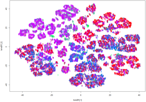
Here, while it is evident that there is some structure and patterns to the data, clustering by OutcomeType has not happened.
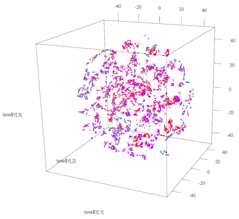
Let’s now use t-SNE to perform dimensionality reduction to 3D on the same dataset. We just need to set the dims parameter to 3 instead of 2. And we will use package rgl for plotting the 3D map produced by t-SNE.
tsne <- Rtsne(trn[,-1], check_duplicates = FALSE, pca = FALSE, perplexity=50, theta=0.5, dims=2)

#display results of t-SNE
require(rgl)
plot3d(tsne$Y, col=cols[trn[,1]])
legend3d("topright", legend = '0':'5', pch = 16, col = rainbow(5))
This 3D map has a richer structure than the 2D version, but again the resulting clustering is not done by OutcomeType.
One possible reason could be that the Manifold Assumption is failing for this dataset when trying to reduce to 2D and 3D. Please note that the Manifold Assumption cannot be always true for a simple reason. If it were, we could take an arbitrary set of \(N\)-dimensional points and conclude that they lie on some \(M\)-dimensional manifold (where \(M < N\)). We could then take those \(M\)-dimensional points and conclude that they lie on some other lower-dimensional manifold (with, say, \(K\) dimensions, where \(K < M\)). We could repeat this process indefinitely and eventually conclude that our arbitrary \(N\)-dimensional dataset lies on a 1D manifold. Because this cannot be true for all datasets, the manifold assumption cannot always be true. In general, if you have \(N\)-dimensional points being generated by a process with \(N\) degrees of freedom, your data will not lie on a lower-dimensional manifold. So probably the Animal Shelter dataset has degrees of freedom higher than 3.
So we can conclude that t-SNE did not aid much the initial exploratory analysis for this dataset.
t-SNE and machine learning?
One disadvantage of t-SNE is that there is currently no incremental version of this algorithm. In other words, it is not possible to run t-SNE on a dataset, then gather a few more samples (rows), and “update” the t-SNE output with the new samples. You would need to re-run t-SNE from scratch on the full dataset (previous dataset + new samples). Thus t-SNE works only in batch mode.
This disadvantage appears to makes it difficult for t-SNE to be used in a machine learning system. But as we will see in a future post, it is still possible to use t-SNE (with care) in a machine learning solution. And the use of t-SNE can improve classification results, sometimes markedly. The limitation is the extra non-realtime processing brought about by t-SNE’s batch mode nature.
Stay tuned.
