Decision Tree falls under supervised machine learning, as the name suggests it is a tree-like structure that helps us to make decisions based on certain conditions. A decision tree can help us to solve both regression and classification problems.
What is Classification?
Classification is the process of dividing the data into different categories or groups by giving certain labels. For Example; categorize the transaction data based on whether the transaction is Fraud or Genuine. If we take the present epidemic as an example based on the symptoms like fever, cold and cough we categorize the patient as suffering from covid or not.
What is Regression?
Regression is a process to get the predictions which is a continuous value. For example; prediction the weight or predicting the sales or profit of the company etc.
A gentle introduction to the Decision tree:
A decision tree is a graphical representation that helps us to make decisions based on certain conditions.
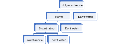
For Example; making a decision whether to watch a movie or not.
Important terminology in the decision tree:
Node:
A decision tree is made up of several nodes:
1.Root Node: A Root Node represents the entire data and the starting point of the tree. From the above example the
First Node where we are checking the first condition, whether the movie belongs to Hollywood or not that is the
Rood node from which the entire tree grows
2.Leaf Node: A Leaf Node is the end node of the tree, which can’t split into further nodes.
From the above example ‘watch movie’ and ‘Don’t watch ‘are leaf nodes.
3.Parent/Child Nodes: A Node that splits into a further node will be the parent node for the successor nodes. The
nodes which are obtained from the previous node will be child nodes for the above node.
Branches:
Branches are the arrows which is a connection between nodes, it represents a flow from the starting/Root node to the leaf node.
How to select an attribute to create the tree or split the node:
We use criteria to select attribute which helps us to split the data into partitions.
Here are the most important and useful methods to select the node for splitting the data
Information Gain:
In the process of selecting an attribute that gives more information about the data, we select the attribute for splitting further from which we get the highest information gain. For calculating Information gain we use matric
Entropy.
Information from attribute = ∑p(x). Entropy (x)
Here, x represents a class in the attribute
Information Gain for any attribute = total entropy – Information from attribute after splitting
Entropy:
Entropy is used to measure the Impurity and disorder in the dataset
Entropy = – ∑ p(y). log2 p(y)
Here, y represents the class in the target variable
Gini Index:
Gini Index is also called Gini Impurity which calculates the probability of an attribute that is randomly selected.
R code
The dataset that we are looking into:
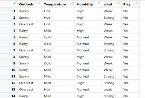
We are going to build a decision tree model to decide whether to play outside or not.
Now we will build a decision tree on the above dataset.
To build a decision tree, first we have to select an attribute that gives highest information among all the attributes.
Calculating Total Entropy
View(dataset)
## changing the data into factors type
data = data.frame(lapply(dataset,factor))
summary(data) ## summary of the data
### Claculating Total Entropy
table(data$Play)
## p(Yes)*log2 p(Yes)-p(No)*log2 p(No)
TotalEntropy= -(9/14)*log2(9/14)-(5/14)*log2(5/14)
TotalEntropy
> View(dataset)
> ## changing the data into factors type
> data = data.frame(lapply(dataset,factor))
> summary(data) ## summary of the data
     Outlook  Temperature   Humidity     wind    Play
 Overcast:4   Cold:4      High  :7   Strong:6   No :5
 Rainy   :5   Hot :4      Normal:7   Weak  :8   Yes:9
 Sunny   :5   Mild:6
> ### Claculating Total Entropy
> table(data$Play)

 No Yes
  5   9
> ## p(Yes)*log2 p(Yes)-p(No)*log2 p(No)
> TotalEntropy= -(9/14)*log2(9/14)-(5/14)*log2(5/14)
> TotalEntropy
[1] 0.940286
Calculate Entropy for each class in Outlook and Information Gain for the Outlook
table(data$Play)
## p(Yes)*log2 p(Yes)-p(No)*log2 p(No)
TotalEntropy= -(9/14)*log2(9/14)-(5/14)*log2(5/14)
TotalEntropy
## filtering Outlook data to calculate entropy
library(dplyr)
## Calculate Entropy for Outlook
Outlook_Rainy = data.frame(filter(select(data,Outlook,Play),Outlook=='Rainy'))

View(Outlook_Rainy)
Entropy_Rainy = -(3/5)*log2(3/5)-(2/5)*log2(2/5)
Entropy_Rainy

Outlook_Overcast = data.frame(filter(select(data,Outlook,Play),Outlook=='Overcast'))
View(Outlook_Overcast)
Entropy_Overcast=-(4/4)*log2(4/4)-0 ## since we don't have any No values
Entropy_Overcast

Outlook_Sunny = data.frame(filter(select(data,Outlook,Play),Outlook=='Sunny'))
View(Outlook_Sunny)
Entropy_Sunny = -(2/5)*log2(2/5)-(3/5)*log2(3/5)
Entropy_Sunny

# calculating Information for outlook
### Info = summation(p(x)*Entropy(x))

Outlook_Info = ((5/14)*Entropy_Rainy)+((4/14)*Entropy_Overcast)+((5/14)*Entropy_Sunny)
Outlook_Info
## Information gain
## Info_gain = Total Entropy- Outlook_info
Info_gain1 = TotalEntropy - Outlook_Info
Info_gain1
> table(data$Play)

 No Yes
  5   9
> ## p(Yes)*log2 p(Yes)-p(No)*log2 p(No)
> TotalEntropy= -(9/14)*log2(9/14)-(5/14)*log2(5/14)
> TotalEntropy
[1] 0.940286
> ## filtering Outlook data to calculate entropy
> library(dplyr)
> ## Calculate Entropy for Outlook
> Outlook_Rainy = data.frame(filter(select(data,Outlook,Play),Outlook=='Rainy'))
> View(Outlook_Rainy)
> Entropy_Rainy = -(3/5)*log2(3/5)-(2/5)*log2(2/5)
> Entropy_Rainy
[1] 0.9709506
> Outlook_Overcast = data.frame(filter(select(data,Outlook,Play),Outlook=='Overcast'))
> View(Outlook_Overcast)
> Entropy_Overcast=-(4/4)*log2(4/4)-0 ## since we don't have any No values
> Entropy_Overcast
[1] 0
> Outlook_Sunny = data.frame(filter(select(data,Outlook,Play),Outlook=='Sunny'))
> View(Outlook_Sunny)
> Entropy_Sunny = -(2/5)*log2(2/5)-(3/5)*log2(3/5)
> Entropy_Sunny
[1] 0.9709506
> Outlook_Info = ((5/14)*Entropy_Rainy)+((4/14)*Entropy_Overcast)+((5/14)*Entropy_Sunny)
> Outlook_Info
[1] 0.6935361
> ## Information gain
> ## Info_gain = Total Entropy- Outlook_info
> Info_gain1 = TotalEntropy - Outlook_Info
> Info_gain1
[1] 0.2467498
Same way calculating entropy and Information gain for all remaining columns
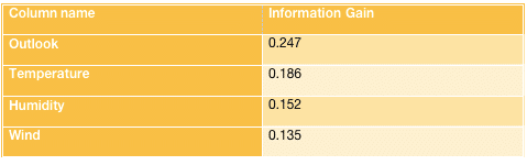
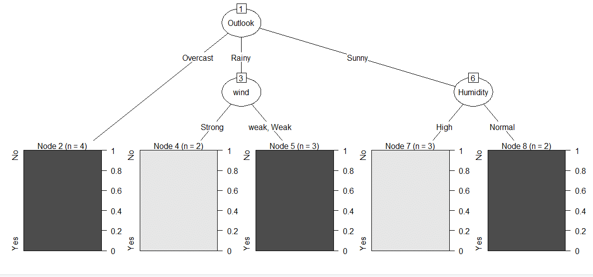
From the Above table Outlook has highest information gain, so the first attribute at the root node is Outlook
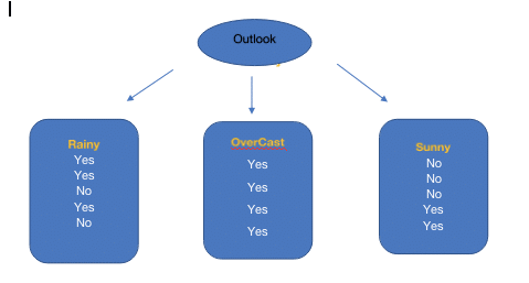
From the above diagram, we can observe that Overcast has only the Yes class. So, there is no need for further splitting. But for the Rainy and Sunny Contains both Yes and No. Again the same process repeats.
Till now, we have seen the manual process
Here is the R code for Building a Decision Tree Model using C5.0 function and plot of the Decision Tree.
library(C50)

## Syntax  C5.0(Input_Columns, Target)

model = C5.0(data[,1:4],data$Play)
plot(model)
Resource Article: simple-linear-regression