Extract Twitter Data Automatically using Scheduler R package

The following R-script is to download the data automatically from Twitter using the package SchedulerR. As first step we download the data using the OAuth protocol and store the data using as a name the date from the download. As second we used the package SchedulerR for to specify how long the script runs. This package has the advantage that we can set the time and also how long will repeat either daily, weekly or monthly.

Load the packages:

library(twitteR)
library(httr)
library(SchedulerR) 

Also we choose the directory where the RData would be saved:

setwd("C:/Users/Documents/schedulerR")

OAuth protocol:

api_key <- "xxxxxxxxxxxxxxxxxxxxxx"
api_secret <- "xxxxxxxxxxxxxxxxxxxxxxxxxxxxxxxxxx"
access_token <- "xxxxxxxxxxxxxxxxxxxxxxxxxxxxxxxx"
access_token_secret <- "xxxxxxxxxxxxxxxxxxxxxxxxxxxxxxxxxxxxxx"
setup_twitter_oauth(api_key,api_secret,access_token,access_token_secret)

Extract the tweets using usertimeline function from the Twitter R package:

 clinton_tweets <- userTimeline("HillaryClinton", n = 3200)
tweetsc.df <- twListToDF(clinton_tweets)
dim(tweetsc.df)

Create a variable called date and become to character:

date<-Sys.Date()
date<-as.character(date)
name<-paste(date,".RData")
#Finally we save the Rdata using as name the date from the download
save(tweetsc.df, file =name)

The script above is to download the data from Twitter. The next step is to use the package SchedulerR::

taskscheduler_create(taskname = "taskclinton", rscript = clintontweets, 
  schedule = "DAILY", starttime = "11:30", startdate = format(Sys.Date(), "%d/%m/%Y")) 

Examples of Analysis

We can implement many analysis from text data.

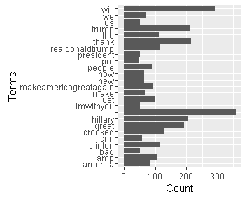
Find words common with a minimun frequency of 45:

term.freq <- rowSums(as.matrix(tdm))
term.freq = 45)
#we saved the data in a data frame
df <- data.frame(term = names(term.freq), freq = term.freq)
save(df,file="tqfclinton50.RData")
#plot with ggplot2
library(ggplot2)
ggplot(df, aes(x = term, y = freq)) + geom_bar(stat = "identity") +
xlab("Terms") + ylab("Count") + coord_flip()

This is the plot:

Hierarchical cluster:

# remove the parse terms
tdm2 <- removeSparseTerms(tdm, sparse = 0.95)
m2 <- as.matrix(tdm2)
# hierarchical cluster
m <- as.matrix(m2)
d<- dist(m2)
#we used the cosine similaruty as distance because is the best option for text data
distcos<-dissimilarity(x=m2,method='cosine')
groups <- hclust(distcos,method="complete")
#plot dendograma
plot(groups, hang=-1)
rect.hclust(groups,5)

This is the plot:

K means clustering

We combine the Kmeans clustering with Principal components analysis to obtain a better result. As a first we used the elbow method for choose the “K”.

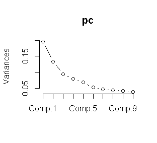
We choose K=5 from the plot. Now we proceed to make the K means clustering.

pc <- princomp(tdm)
plot(pc)
data<-tdm
wss <- (nrow(data)-1)*sum(apply(data,2,var))
for (i in 2:15) wss[i] <- sum(kmeans(data,
centers=i)$withinss)
plot(1:15, wss, type="b", xlab="Number of Clusters",
ylab="Within groups sum of squares")

m3 <- t(tdm2) # transpse from term document matriz
set.seed(1222) # we choose a seed.
k <- 5# number of clusters
kmeansResult <- kmeans(m3, k)
km<-round(kmeansResult$centers, digits = 3) 
#we saved in a csv file.
write.csv(km,file="kmeansclinton.csv")

The following loop is for visualize the clusters.

for (i in 1:k) {
cat(paste("cluster ", i, ": ", sep = ""))
s <- sort(kmeansResult$centers[i, ], decreasing = T)
cat(names(s)[1:5], "\n")
}
write.csv(s,file="clusterkm.csv")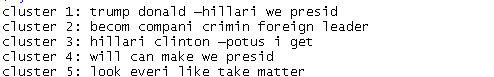  

Based in the results we can say from each cluster they are the topics most words used in the tweets.