Regression is one of the – maybe even the single most important fundamental tool for statistical analysis in quite a large number of research areas. It forms the basis of many of the fancy statistical methods currently en vogue in the social sciences. Multilevel analysis and structural equation modeling are perhaps the most widespread and most obvious extensions of regression analysis that are applied in a large chunk of current psychological and educational research. The reason for this is that the framework under which regression can be put is both simple and flexible. Another great thing is that it is easy to do in R and that there are a lot – a lot – of helper functions for it.
Let’s take a look at an example of a simple linear regression. I’ll use the swiss dataset which is part of the datasets-Package that comes pre-packaged in every R installation. To load it into your workspace simply use
data(swiss)Copy
As the helpfile for this dataset will also tell you, its Swiss fertility data from 1888 and all variables are in some sort of percentages. The outcome I’ll be taking a look at here is the Fertility indicator as predictable by the education beyond primary school – my basic assumption being that higher education will be predictive of lower fertility rates (if the 1880s were anything like today).
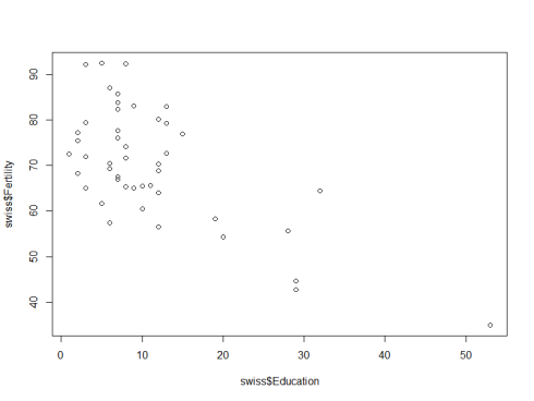
First, lets take a look at a simple scatterplot:
plot(swiss$Fertility~swiss$Education)Copy
The initial scatterplot already suggests some support for the assumption and – more importantly – the code for it already contains the most important part of the regression syntax. The basic way of writing formulas in R is dependent ~ independent. The tilde can be interpreted as “regressed on” or “predicted by”. The second most important component for computing basic regression in R is the actual function you need for it: lm(...), which stands for “linear model”.
The two arguments you will need most often for regression analysis are the formula and the data arguments. These are incidentally also the first two of the lm(...)-function. Specifying the data arguments allows you to include variables in the formula without having to specifically tell R where each of the variables is located. Of course, this only works if both variables are actually in the dataset you specify. Let’s try it and assign the results to an object called reg
reg <- lm(Fertility~Education,swiss)
reg
Call:
lm(formula = Fertility ~ Education, data = swiss)

Coefficients:
(Intercept)    Education
    79.6101      -0.8624
Copy
The basic output of the lm(...) function contains two elements: the Call and the Coefficients. The former is used to tell you what regression it was that you estimated – just to be sure – and the second contains the regression coefficients. In this case there are two coefficients: the intercept and the regression weight of our sole predictor. What this tells us is that for a province with an educational value of 0 a fertility value of 79.61 is predicted. This is often also called a condtional expectation because it is the value you expect for the dependent variable under the condition that the independent variable is 0. Put a bit more formally: $latex E(Y|X=0) = 79.61$. The regression weight is the predicted difference between two provinces that differ in education by a single point.
Like for most R objects, the summary-function shows the most important information in a nice ASCII table.
summary(reg)
Call:
lm(formula = Fertility ~ Education, data = swiss)

Residuals:
    Min      1Q  Median      3Q     Max
-17.036  -6.711  -1.011   9.526  19.689

Coefficients:
            Estimate Std. Error t value Pr(>|t|)
(Intercept)  79.6101     2.1041  37.836  < 2e-16 ***
Education    -0.8624     0.1448  -5.954 3.66e-07 ***
---
Signif. codes:  0 ‘***’ 0.001 ‘**’ 0.01 ‘*’ 0.05 ‘.’ 0.1 ‘ ’ 1

Residual standard error: 9.446 on 45 degrees of freedom
Multiple R-squared:  0.4406,	Adjusted R-squared:  0.4282
F-statistic: 35.45 on 1 and 45 DF,  p-value: 3.659e-07
Copy
What is the most important information in this table? Most probably the coefficients-section, which contains the parameter estimates and their corresponding t-tests. This shows us that the education level in a province is significantly related to the fertility rate in.
The second most important line is the one containing the $latex R^2$. In this case over 44% of the provincial variability in fertility is shared with the variability in the educational level. Due to the fact that the $latex R^2$ is the squared multiple correlation between the dependent and all independent variables the square of the Pearson-Correlation the correlation between fertility and education should be exactly equal to the $latex R^2$ we found here. To check this, we can use
summary(reg)$r.squared
cor(swiss$Fertility,swiss$Education)^2
summary(reg)$r.squared == cor(swiss$Fertility,swiss$Education)^2
0.4406156
0.4406156
TRUE
Copy
The last line of this code performs the logical check for identity of the two numbers.
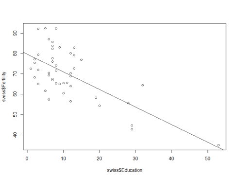
To wrap up, we’ll add the regression line to the scatterplot we generated at the beginning of this post. As noted, the lm(...)-function and its results are extremely well embedded in the R environment. So all we need to add the resulting regression line is the abline(...)-function. This function can be used to add any line which can be described by an intercept (a) and a slope (b). If you provide an object of the lm-class, the regression line will be drawn for you.
plot(swiss$Fertility~swiss$Education)
abline(reg)
Copy
This wraps up the very basic introduction to linear regression in R. In future post we’ll extend these concepts to multiple regression and take a look at how to easily check for the assumptions made in OLS regression.

